조범희 선생님의 선형대수학개론 강의를 듣고 공부하며 정리한 내용입니다.
정말 좋은 강의힙니다. 강추합니다. 링크
Homogeneous Linear Systems
A x = 0
always has at least one solution x = 0
trivial solution - 너무 당연한 solution 이라서 그런지 trivial solution 이라고 함
nontrivial solution
if and only if the equation has at least one free variable (by Theorem2.)
Example1. Determine whether there is a nontrivial solution
3x1+5x2−4x3=0−3x1−2x2+4x3=06x1+x2−8x3=0
이 문제를 풀어보면 x3 가 free variable 로 나타난다 (infinite number of solutions)
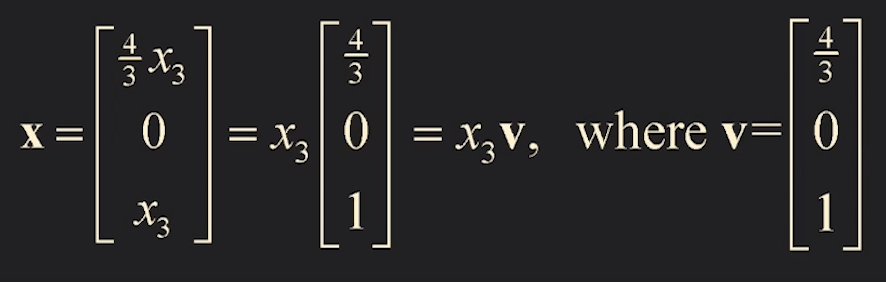
이러한 꼴이 되는데
이는 즉, Span { v } 이다 (vector v 에 x1이라는 scalar 값이 scalar multiplication 된 것이므로)
그리고 다시, 이는 Line 임을 말해준다 ( R3 에서 span { v } 는 line 이므로)
Example 2. Determine whether there is a nontrivial solution
10x1−3x2−2x3=0
x=⎣⎢⎡0.3x2+0.2x3x2x3⎦⎥⎤⎣⎢⎡0.3x2x20⎦⎥⎤+⎣⎢⎡0.2x30x3⎦⎥⎤=x2⎣⎢⎡0.310⎦⎥⎤+x3⎣⎢⎡0.201⎦⎥⎤
→ Span {u,v}
→ plane!
따라서,
A x = 0
-
the solution set can always be expressed as Span {v1,⋯,vp}
-
trivial solution is Span {0}
Nonhomogeneous Linear Systems
Example 3. Describe all solutions of A x = b
A=⎣⎢⎡3−365−21−44−8⎦⎥⎤b=⎣⎢⎡7−1−4⎦⎥⎤
이때의 A는 Example 1.과 동일하다
Example 1.에서는 Span{v},v=(34,0.1) 이었는데 이를 유념해서 이 문제의 결과를 지켜보자
Solution.
⎣⎢⎡3−365−21−44−87−1−4⎦⎥⎤∼⎣⎢⎡100010−3400−120⎦⎥⎤
으로
x=⎣⎢⎡−1+34x32x3⎦⎥⎤=⎣⎢⎡−120⎦⎥⎤+x3⎣⎢⎡3401⎦⎥⎤ 이 된다
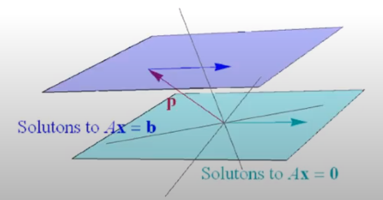
이는 x=p+x3v=p+tv 가 된다.
(p = particular solution으로, Ax=b의 solution 중 특정한 하나의 solution이고,
v = homogeneous solution 으로, Ax=0 의 모든 solution 이다.)
Theorem 6.
Suppose Ax=b is consistent (has a solution),
and let p be a solution (Ap=b)
Then the solution set of Ax=b is the set of all vectors of the form
w=p+vh
where vh is any solution of the homogeneous equation Ax=0
Example 4. Understanding Theorem 6. in R3
(proof 와 visualization 은 링크 를 참고했다)
Theorem 6.를 증명하려면,
1) p+vh 꼴의 vector 가 Ax=b 의 해이면서
2) Ax=b의 모든 해가 p+vh의 꼴을 가지면 된다
이렇게 되면 'p+vh 꼴의 벡터'와 'Ax=b의 모든 해' 라는 두 집합이 서로의 부분집합이 되면서, 두 집합은 동치이게 되고 이는 즉, Theorem 6과 같아진다
(다시 상기하자면, p = particular solution으로, Ax=b의 solution 중 특정한 하나의 solution이고,
v = homogeneous solution 으로, Ax=0 의 모든 solution 이다.)
1)는 간단하다.
A(p+vh)=Ap+Avh=b+0=b
로 간단하게 해결이 된다.
(2)를 해결해보자
Ax=b의 해인 s 가 있다고 가정하자.
그렇다면 s−p는
A(s−p)=As−Ap=b−b=0 으로 인해
Ax=0 의 해이다.
즉, s−p=vh 이므로, s=p+vh 꼴이 된다.
즉 (2)가 해결됐다
따라서, Theorem 6. 은 참이다.
조범희 선생님의 visualization보다 이 유튜브의 visualization이 조금 더 잘 이해됐는데,
p가 particular solution 이므로 고정된 vector로 놓고, vh는 homogeneous system의 all solution이니 계속 변화하는 벡터로 생각할 수 있다.
이때 vh가 직선이라고 생각하면, w는 vh와 평행한 직선으로 나타나게 되는 것을 알 수 있다.
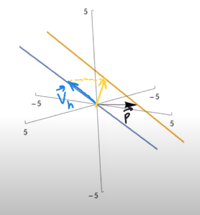
이를 일반화하면, 2차원에서 Theorem 6를 visualize 할 수 있다.