[CS224W] 2. Traditional Methods for Machine Learning in Graphs

🔨 Machine Learning Tasks

• Node-level prediction
• Link-level prediction
• Graph-level prediction
  
  

🔨 Traditional ML Pipleline

• Design features for nodes/links/graphs
• Obtain features for all training data

1. Train an ML model
Data point, node, link, graph 등을 feature Vector로 변환해 ML model을 학습시킨다
2. Apply the model
새로운 입력이 들어오면 feature Vector를 얻고 모델을 통해 예측한다.

🔨 Feature Design

Using effective features over graph !!

✔️ Goal : 입력 Set이 주어졌을 때 예측 값을 만들어내는 것
✔️ Design choices
[] Features : d 차원의 벡터
[] Objects : Nodes, Links, Sets of Nodes, Entire Graph
[] Objective : 우리가 풀려고 하는 task

📁 Node-Level Features

Goal : Characterize the structure and position of a node in the network

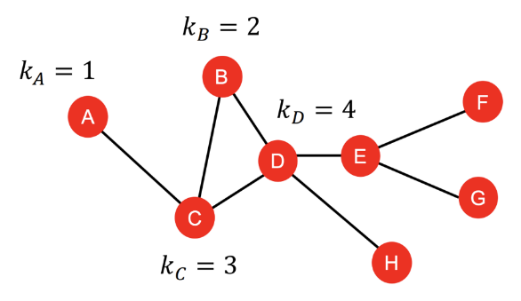
✔️ 1. Node degree (kv)

• kv = Node v의 degree
• kv = v가 가지고 있는 Edge(Link)의 수
  

✔️ 2. Node centrality (cv)

• Node Degree는 이웃한 Node의 개수만 셀 뿐, 중요도(importance)를 caputure할 수 없다.
• Node Centrality는 Graph에서 해당 Node v의 importance를 포함한다

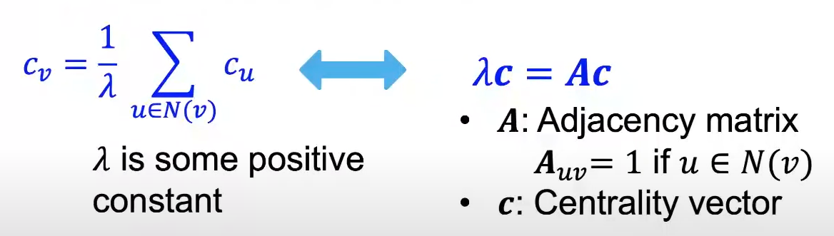
  2-1. Engienvector centrality

• Node v가 Important 이웃노드 u에 둘러싸여있을 때 v는 Important 하다.
  

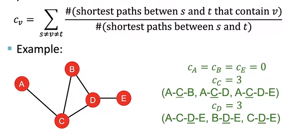
  2-2. Betweenness centrality

• v가 다른 노드들을 연결하는 최단 경로에 있을 때 Important하다고 한다.
  

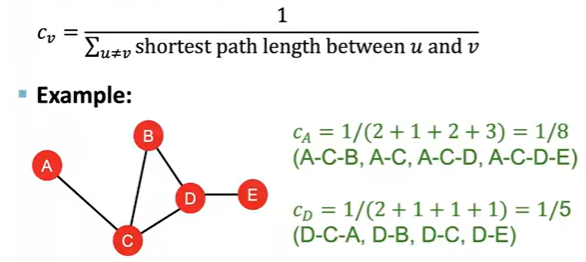
  2-3. Closeness centrality

• v가 다른 모든 노드에 대한 최단 경로의 길이가 짧을 때 Important
  

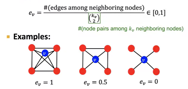
✔️ Clustering coefficient

• Node v의 이웃들이 얼마나 연결되어 있는지를 측정하는 개념
  

✔️ Graphlets

Connected(서로 연결되어 있는) induced non-isomorphic subgraphs
Goal : Node u의 이웃구조를 기술

• induced subgraph : 어떤 노드들을 선택했을 때, 해당 노드들 사이에 연결된 모든 edge들을 포함하는 subgraph
• graph isomorphism : 두 그래프가 같은 개수의 노드를 가지고 있고, 노드들이 똑같이 연결되어 있는 것
  언뜻 보기에 달라보이지만 노드를 잘 매핑하면 edge관계가 같기 때문에 isomorphism grph이다.
  
  

✔️ Graphlet Degree Vector(GDV)

= Node의 Graphelt-Based Feature

• Degree of Graphlet : 특정 Node가 포함된 Graphlet의 개수 벡터

  1. Graph G에서 Node u를 타깃으로 정한 상황
     2. Graph G에서 최대 노드가 3개인 Graphlet 3개를 도출할 수 있다.
     3. 각 Graphlet이 G에서 u를 포함한 채로 몇번 나타나는지 count 4. Node u의 GDV는 [2,1,0,2] 가 된다.

Node-Level Feature Summary

✔️ Importance Based

a. Node Degree : 이웃의 개수 count
b. Node Centrality : Graph에서의 이웃 노드 중요도를 모델링

✔️ Structure Based

a. Node Degree : 이웃의 개수 count
b. Clustering Coefficient : 이웃이 어떻게 연결되어 있는지 측정
c. Graphlet Count Vector : 여러 Graphlet들이 출현하는 빈도를 count

📁 Link-Level Features

✔️ Link-Level Prediction Tast

존재하는 Link를 바탕으로 새로운 Link를 예측하는 것

• 랜덤하게 사라진 Link 찾기 -> Static한 Graph에 적절
• 시간이 흐름에 따라 생겨나는 Link 찾기 -> Dynamic한 Graph에 적절 ex) SNS

✔️ Features

• Distance-Based : 두 Node간 최단 경로의 거리

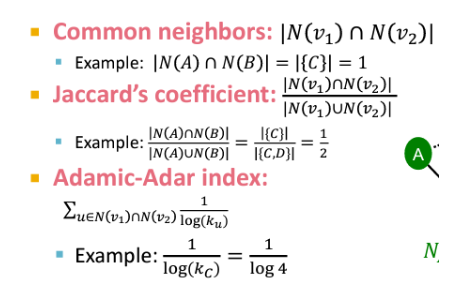
  단점 : neighborhood overlap의 정보는 사용되지 않는다.

• Local Neighborhood Overlap : 두 Node가 공유하는 이웃의 수

  

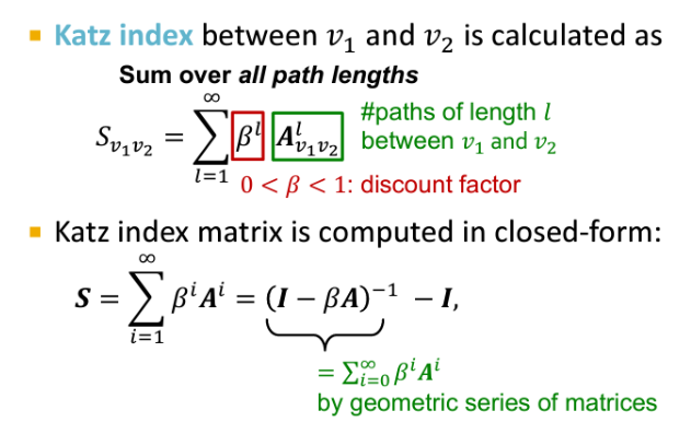
• Global Neighborhood Overlap : 두 Node를 잇는 모든 길의 경로 가중합

  -> 전체 그래프를 고려하여 local neighborhood overlap의 단점을 극복한다
  

📁 Graph-Level Features

Goal : Feature Vector 대신 전체 Graph 구조를 특정할 수 있는 Feature을 만들자

✔️ Features

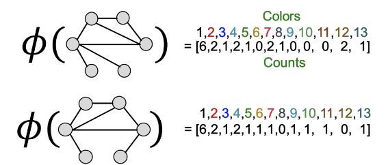
• Graphlet Kernel

  Bag-of-Graphlets로 feature vector을 만든 후 kernel을 계산한다
  단점 : graphlet을 count하는 것이 비싸고, 비효율적이다.
  
  

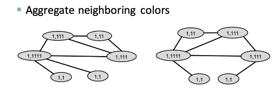
• Weisfeiler-Lehman(WL) Kernel

  장점: efficient, 전체 시간 복잡도 O(# of edges) / GNN과 관련이 크다
• [ Color Refienment ] : After K steps of color refinement, the structure of K-hop neighborhood is summarized
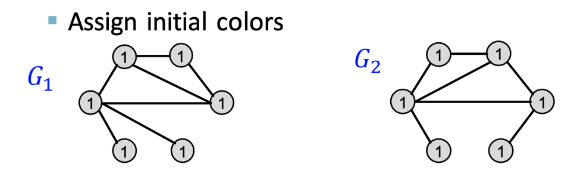
  비슷한 Graph 두개 (G1,G2)가 주어져있다.

1. 동일한 Initial Color를 모든 Node에 할당
   
2. 이웃노드의 색을 Aggregate 해준다
   
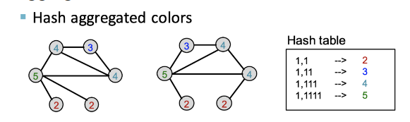
3. Aggregate된 color를 Hash 한다
   
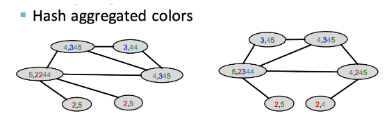
4. 이웃노드 색을 Aggregate 한다
   
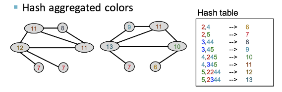
5. Aggregate된 color를 Hash 한다
   
6. Color Fefinement가 끝나면 WL Kernel이 각 Color가 등장한 횟수를 count한다
   
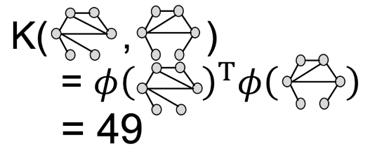
7. Color Count Vector를 내적하여 WL Kernel의 결과값을 구한다
   

Reference

https://www.youtube.com/watch?v=3IS7UhNMQ3U&list=PLoROMvodv4rPLKxIpqhjhPgdQy7imNkDn&index=4