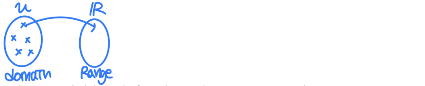
Def: A "random variable" X ( u ) X(u) X ( u ) mapping from the sample space to the real line ;X X X u u u
Mathematically, a random variable is a function from the sample space U U U to real numbers R R R X ( u ) X(u) X ( u ) u u u R R R
We can have several random variables defined on the same sample space
discrete RV / continuous RV Ex_ X X X f i f_i f i i i i ∈ \in ∈ discrete RV
Ex_ U U U X ( u ) X(u) X ( u ) u 2 u^2 u 2 X X X ∈ \in ∈ continuous RV
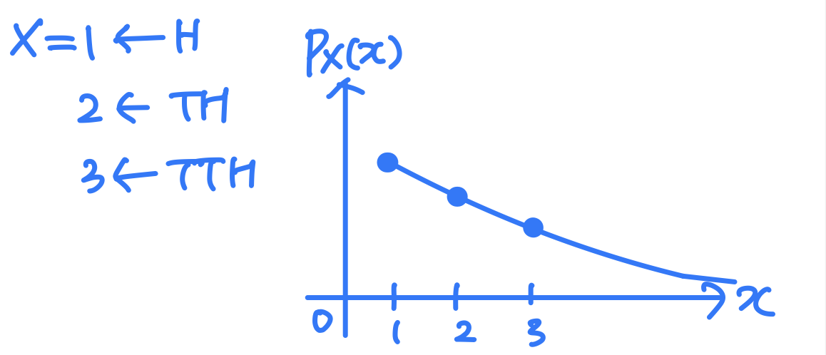
Probability mass function ( PMF )
P X ( x ) = P [ X = x ] P_X(x) = P[X = x] P X ( x ) = P [ X = x ] X X X x x x
Ex_ X ( u ) X(u) X ( u ) P X ( 10 ) P_X(10) P X ( 1 0 ) P X ( 20 ) P_X(20) P X ( 2 0 ) P X ( 60 ) P_X(60) P X ( 6 0 )
used for discrete RVs
P X ( x ) P_X(x) P X ( x ) ≥ \ge ≥ Σ x P X ( x ) \Sigma_xP_X(x) Σ x P X ( x )
Ex_ Binomial random variableP X ( x ) P_X(x) P X ( x ) ( x n ) p x ( 1 − p ) n − x (^n_x)p^x(1-p)^{n-x} ( x n ) p x ( 1 − p ) n − x Binomial PMF "
Ex_ Geometric random variableP X ( x ) P_X(x) P X ( x ) ( 1 − p ) x − 1 p (1-p)^{x-1}p ( 1 − p ) x − 1 p
Probability density function ( PDF )
A continuous RV X X X f X ( x ) f_X(x) f X ( x ) X X X x x x
∫ − ∞ ∞ f X ( x ) d x \int^{\infin}_{-\infin}f_X(x)dx ∫ − ∞ ∞ f X ( x ) d x ∫ a b f X ( x ) d x \int^b_af_X(x)dx ∫ a b f X ( x ) d x P ( X ∈ B ) P(X \in B) P ( X ∈ B ) ∫ B f X ( x ) d x \int_B f_X(x)dx ∫ B f X ( x ) d x P(x x x X X X δ \delta δ ∫ x x + δ f X ( x ) d x \int_x^{x+\delta}f_X(x)dx ∫ x x + δ f X ( x ) d x δ \delta δ ≈ P ( X = x ) \approx P(X=x) ≈ P ( X = x ) ≈ f X ( x ) ∗ δ \approx f_X(x)*\delta ≈ f X ( x ) ∗ δ
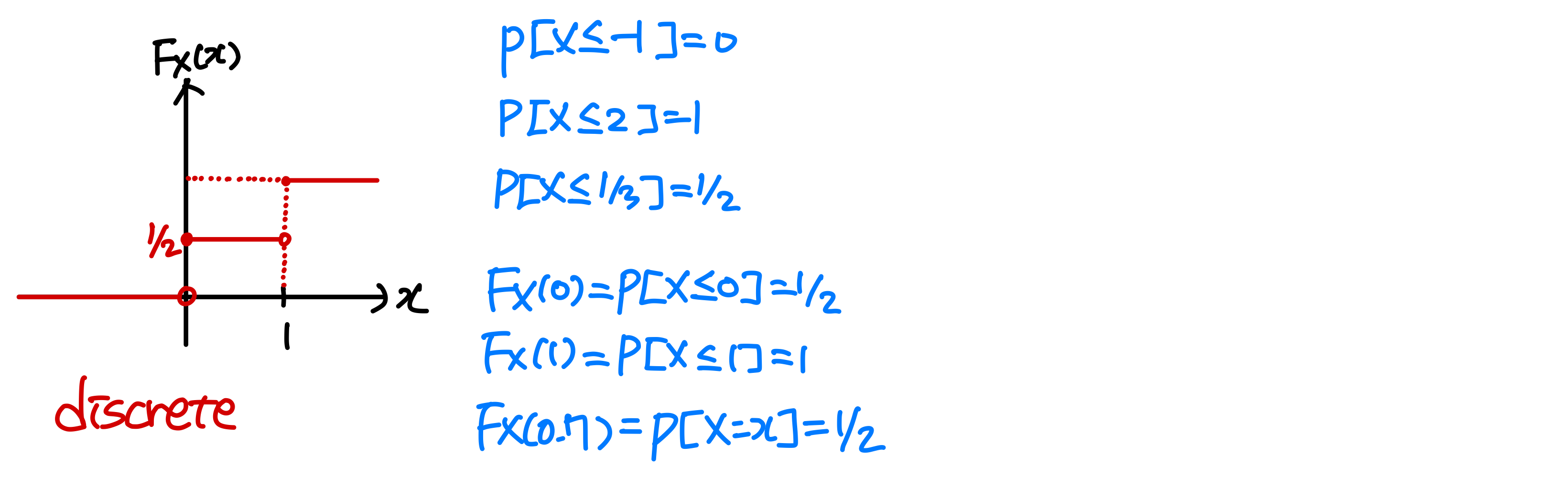
Probability distribution function (Cumulative Distribution Function, CDF)
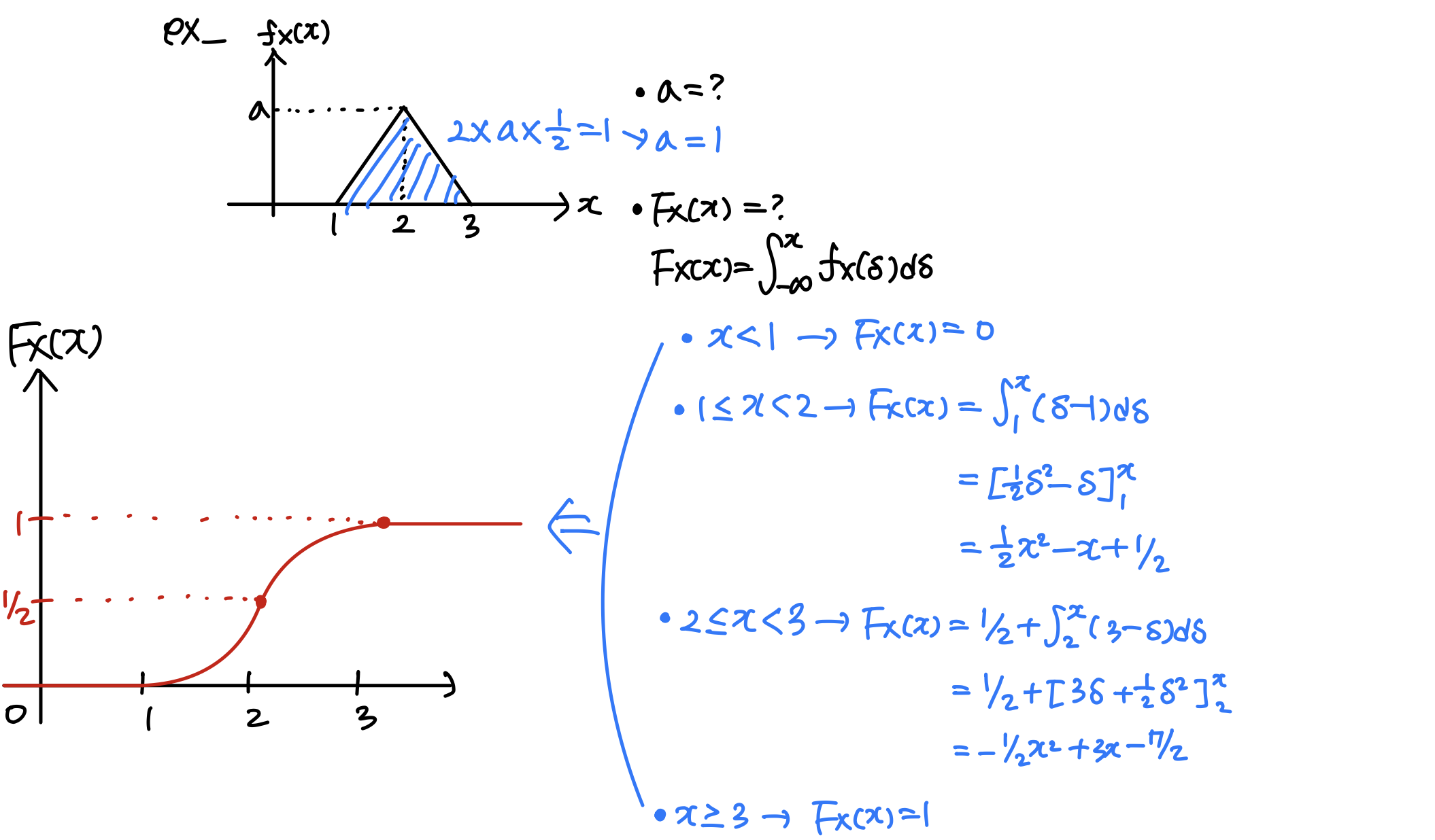
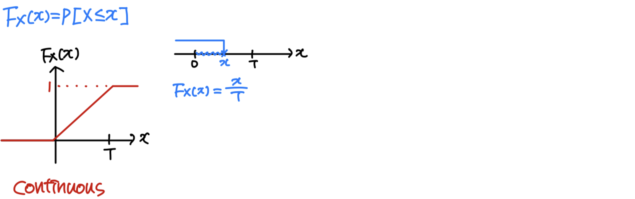
Def: F X ( x ) = P [ X ≤ x ] = ∫ − ∞ x f X ( ζ ) d ζ F_X(x) = P[X≤x] = \int^x_{-\infin}f_X(\zeta)d\zeta F X ( x ) = P [ X ≤ x ] = ∫ − ∞ x f X ( ζ ) d ζ ζ \zeta ζ
f X ( x ) = d d x F X ( x ) f_X(x) = \frac{d}{dx}F_X(x) f X ( x ) = d x d F X ( x )
Ex_ coin tossingX ( h ) = 1 , X ( t ) = 0 X(h) = 1, X(t) = 0 X ( h ) = 1 , X ( t ) = 0 P X ( 1 ) = P X ( 0 ) = 1 / 2 P_X(1) = P_X(0) = 1/2 P X ( 1 ) = P X ( 0 ) = 1 / 2
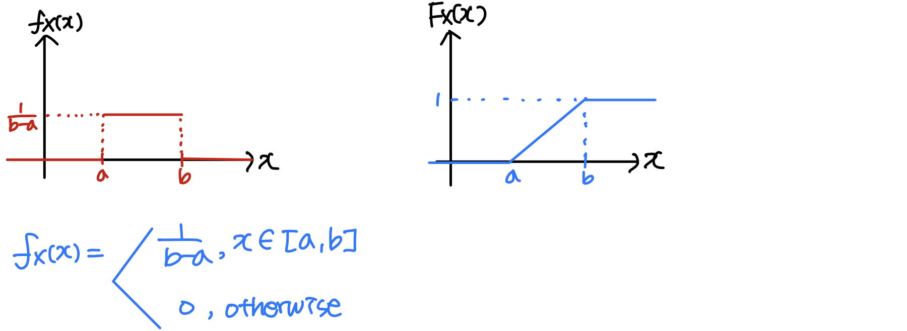
Ex_ A bus arrives at random between (0, T)
Properties of probability distribution function (CDF)
F X ( ∞ ) = P [ X ≤ ∞ ] F_X(\infin) = P[X \le \infin] F X ( ∞ ) = P [ X ≤ ∞ ] 1 F X ( − ∞ ) = P [ X ≤ − ∞ ] F_X(-\infin) = P[X \le -\infin] F X ( − ∞ ) = P [ X ≤ − ∞ ] 0 F X ( x ) F_X(x) F X ( x ) x x x if x 1 < x 2 x_1 < x_2 x 1 < x 2 F X ( x 1 ) ≤ F X ( x 2 ) F_X(x_1) \le F_X(x_2) F X ( x 1 ) ≤ F X ( x 2 ) P [ X > x ] P[X>x] P [ X > x ] 1 − F X ( x ) 1-F_X(x) 1 − F X ( x ) F X ( x ) F_X(x) F X ( x ) right-continuous P [ x 1 < X ≤ x 2 ] P[x_1<X\le x_2] P [ x 1 < X ≤ x 2 ] F X ( x 2 ) − F X ( x 1 ) F_X(x_2)-F_X(x_1) F X ( x 2 ) − F X ( x 1 ) x 2 > x 1 x_2>x_1 x 2 > x 1 X ≤ x 2 X \le x_2 X ≤ x 2 x 1 < X ≤ x 2 x_1 < X \le x_2 x 1 < X ≤ x 2 ∪ \cup ∪ X ≤ x 1 X \le x_1 X ≤ x 1 P [ X ≤ x 2 ] P[X \le x_2] P [ X ≤ x 2 ] P [ x 1 < X ≤ x 2 ] P[x_1 < X \le x_2] P [ x 1 < X ≤ x 2 ] P [ X ≤ x 1 ] P[X \le x_1] P [ X ≤ x 1 ] F X ( x 2 ) F_X(x_2) F X ( x 2 ) P [ x 1 < X ≤ x 2 ] P[x_1 < X \le x_2] P [ x 1 < X ≤ x 2 ] F X ( x 1 ) F_X(x_1) F X ( x 1 ) P [ x 1 < X ≤ x 2 ] = F X ( x 2 ) − F X ( x 1 ) P[x_1 < X \le x_2] = F_X(x_2)-F_X(x_1) P [ x 1 < X ≤ x 2 ] = F X ( x 2 ) − F X ( x 1 ) P [ X = x ] = P [ x − < X ≤ x ] P[X=x] = P[x^-<X\le x] P [ X = x ] = P [ x − < X ≤ x ] = F X ( x ) − F X ( x − ) = F_X(x)-F_X(x^-) = F X ( x ) − F X ( x − )
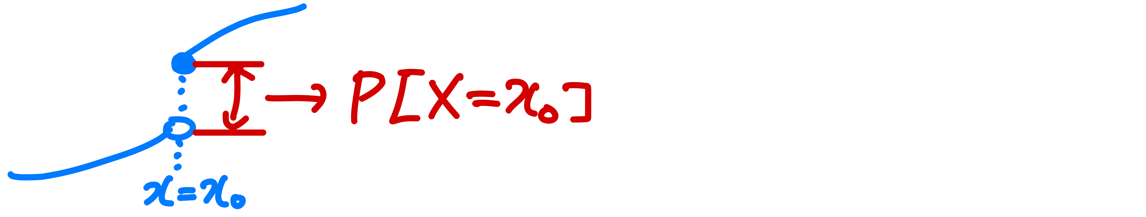
Note_ F X ( x ) F_X(x) F X ( x ) x = x 0 x=x_0 x = x 0 P [ X = x 0 ] = 0 P[X=x_0]=0 P [ X = x 0 ] = 0 F X ( x ) F_X(x) F X ( x ) x = x 0 x=x_0 x = x 0 P [ X = x 0 ] = F X ( x 0 ) − F X ( x 0 − ) P[X=x_0]=F_X(x_0)-F_X(x_0^-) P [ X = x 0 ] = F X ( x 0 ) − F X ( x 0 − )
Comment_ complete Statistical description
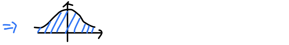
Typical density functions
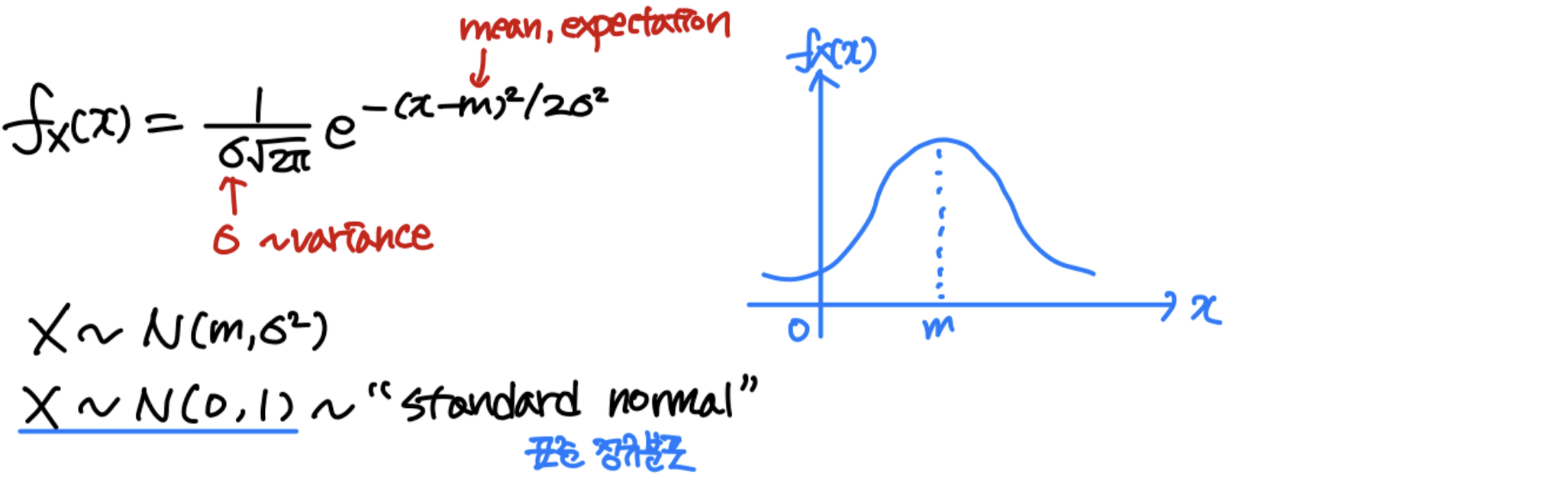
Gaussian ( normal )
X X X N N N m m m σ 2 \sigma^2 σ 2
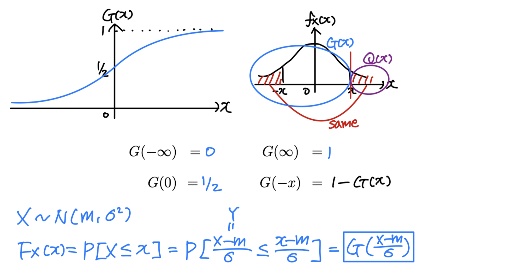
G ( x ) G(x) G ( x ) ∫ − ∞ x 1 2 π e ζ 2 / 2 d ζ \int^x_{-\infin}\frac{1}{\sqrt {2\pi}}e^{\zeta^2/2}d\zeta ∫ − ∞ x 2 π 1 e ζ 2 / 2 d ζ
Q ( x ) = 1 − G ( x ) Q(x) = 1-G(x) Q ( x ) = 1 − G ( x ) Q ( − x ) = 1 − Q ( x ) = G ( x ) Q(-x) = 1-Q(x)=G(x) Q ( − x ) = 1 − Q ( x ) = G ( x ) f X ( x ) = 1 8 π e − ( x + 3 ) 2 / 8 f_X(x)=\frac{1}{\sqrt {8\pi}}e^{-(x+3)^2/8} f X ( x ) = 8 π 1 e − ( x + 3 ) 2 / 8 X X X
P [ ∣ X + 3 ∣ < 2 ] = P [ − 5 < X < − 1 ] P[|X+3|<2] = P[-5<X<-1] P [ ∣ X + 3 ∣ < 2 ] = P [ − 5 < X < − 1 ] F X ( − 1 ) − F X ( − 5 ) F_X(-1)-F_X(-5) F X ( − 1 ) − F X ( − 5 ) G ( − 1 + 3 2 ) − G ( − 5 + 3 2 ) G(\frac{-1+3}{2})-G(\frac{-5+3}{2}) G ( 2 − 1 + 3 ) − G ( 2 − 5 + 3 ) G ( 1 ) − G ( − 1 ) G(1)-G(-1) G ( 1 ) − G ( − 1 ) G ( 1 ) − 1 + G ( 1 ) G(1)-1+G(1) G ( 1 ) − 1 + G ( 1 ) 2 G ( 1 ) − 1 2G(1)-1 2 G ( 1 ) − 1 1 − 2 Q ( 1 ) 1-2Q(1) 1 − 2 Q ( 1 )
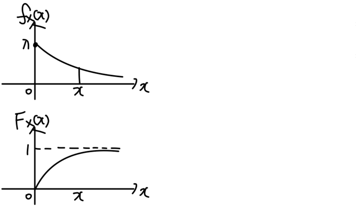
Exponential
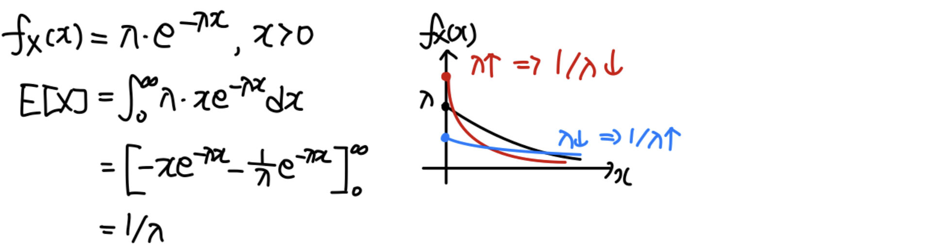
f X ( x ) = λ e − λ x , x ≥ 0 f_X(x)=\lambda e^{-\lambda x},x\ge0 f X ( x ) = λ e − λ x , x ≥ 0 = 0 =0 = 0
F X ( x ) = ∫ 0 x λ e − λ ζ d ζ F_X(x) = \int^x_0\lambda e^{-\lambda \zeta}d\zeta F X ( x ) = ∫ 0 x λ e − λ ζ d ζ = [ − e − λ ζ ] 0 x = [-e^{-\lambda \zeta}]^x_0 = [ − e − λ ζ ] 0 x = 1 − e − λ x , x ≥ 0 = 1-e^{-\lambda x}, x\ge0 = 1 − e − λ x , x ≥ 0
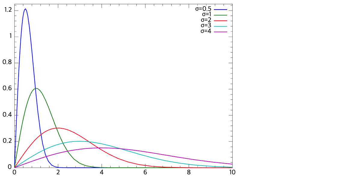
Rayleigh
f X ( x ) = x σ 2 e − x 2 / 2 σ 2 , x ≥ 0 f_X(x) = \frac{x}{\sigma^2}e^{-x^2/2\sigma^2}, x\ge0 f X ( x ) = σ 2 x e − x 2 / 2 σ 2 , x ≥ 0
Poisson
단위 시간 안에 어떤 사건이 몇 번 발생할 것인지를 표현
Discrete RV
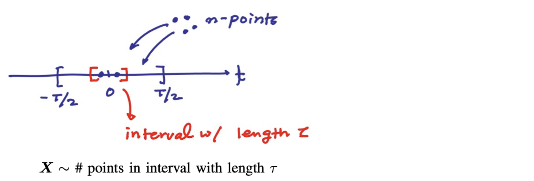
Consider a random point experiment
P X ( k ) = ( n k ) p k q n − k P_X(k) = (^k_n)p^kq^{n-k} P X ( k ) = ( n k ) p k q n − k p = τ T p=\frac{\tau}{T} p = T τ q = 1 − τ T q=1-\frac{\tau}{T} q = 1 − T τ Assume T → ∞ \infin ∞ ∞ \infin ∞ λ \lambda λ
P X ( k ) ≅ e − λ τ ( λ τ ) k k ! P_X(k) \cong e^{-\lambda\tau}\frac{(\lambda\tau)^k}{k!} P X ( k ) ≅ e − λ τ k ! ( λ τ ) k
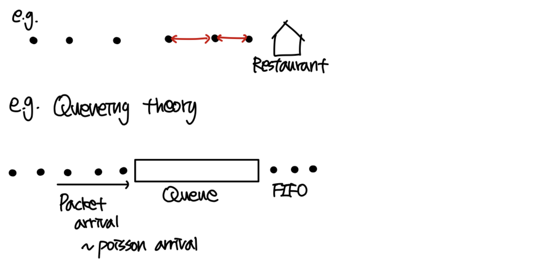
Q: What is the density of distance between adjacent points?F Y ( y ) = P [ Y ≤ y ] F_Y(y)=P[Y\le y] F Y ( y ) = P [ Y ≤ y ] P [ Y > y ] = P [ P[Y>y]=P[ P [ Y > y ] = P [ ] ] ] 1 − F Y ( y ) = e − λ y , y ≥ 0 1-F_Y(y)=e^{-\lambda y},y\ge0 1 − F Y ( y ) = e − λ y , y ≥ 0 ∴ F Y ( y ) = 1 − e − λ y , y ≥ 0 \therefore F_Y(y) = 1-e^{-\lambda y}, y\ge0 ∴ F Y ( y ) = 1 − e − λ y , y ≥ 0 f Y ( y ) = λ e − λ y , y ≥ 0 f_Y(y) = \lambda e^{-\lambda y}, y\ge0 f Y ( y ) = λ e − λ y , y ≥ 0
Expectation
Definition
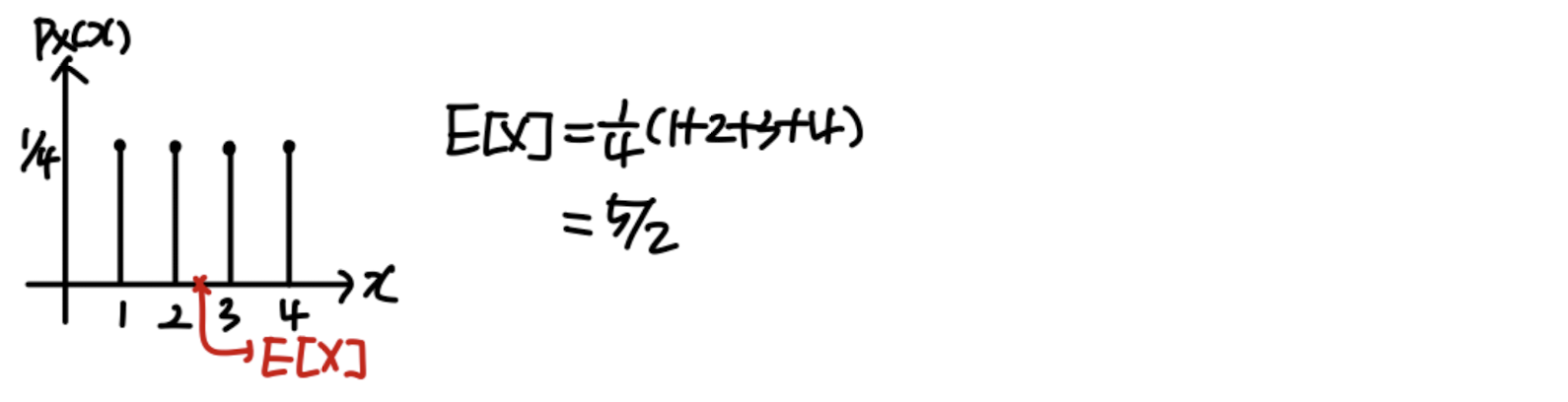
For a discrete RV, E [ X ] = ∑ x x P X ( x ) E[X] = \sum_x xP_X(x) E [ X ] = ∑ x x P X ( x )
Indicates the center of gravity
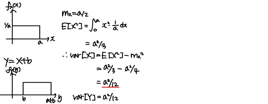
e.g. uniform RV
For a continuous. RV, E [ X ] = ∫ − ∞ ∞ x f X ( x ) d x E[X]=\int^\infin_{-\infin}xf_X(x)dx E [ X ] = ∫ − ∞ ∞ x f X ( x ) d x
e.g. exponential RV
Expectation of a function of a RV
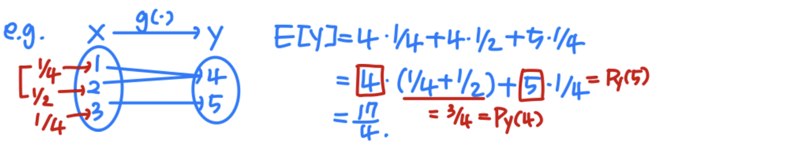
Let Y = g ( X ) Y=g(X) Y = g ( X ) Y Y Y
For a discrete RV, E [ Y ] = ∑ y y P Y ( y ) = ∑ x g ( x ) P X ( x ) E[Y]=\sum_yyP_Y(y) = \sum_xg(x)P_X(x) E [ Y ] = ∑ y y P Y ( y ) = ∑ x g ( x ) P X ( x )
Similary, for a continuous RV, E [ Y ] = ∫ − ∞ ∞ g ( x ) f X ( x ) d x E[Y]=\int^\infin_{-\infin}g(x)f_X(x)dx E [ Y ] = ∫ − ∞ ∞ g ( x ) f X ( x ) d x
Properties
E [ − ] E[-] E [ − ] E [ a X ] = a E [ X ] E[aX]=aE[X] E [ a X ] = a E [ X ] E [ a X + b ] = a E [ X ] + b E[aX+b]=aE[X]+b E [ a X + b ] = a E [ X ] + b In general, E [ g ( X ) ] ≠ g ( E [ X ] ) E[g(X)]\neq g(E[X]) E [ g ( X ) ] = g ( E [ X ] )
e.g. g ( X ) = x 2 g(X) = x^2 g ( X ) = x 2 E [ X 2 ] ≠ E 2 [ X ] E[X^2]\neq E^2[X] E [ X 2 ] = E 2 [ X ]
Variance
V a r [ X ] = E [ ( X − m x ) 2 ] Var[X] = E[(X-m_x)^2] V a r [ X ] = E [ ( X − m x ) 2 ] = ∫ − ∞ ∞ ( x − m x ) 2 f X ( x ) d x = \int^\infin_{-\infin}(x-m_x)^2f_X(x)dx = ∫ − ∞ ∞ ( x − m x ) 2 f X ( x ) d x σ X 2 = E [ X 2 ] − m x 2 \sigma^2_X = E[X^2]-m_x^2 σ X 2 = E [ X 2 ] − m x 2 σ X = V a r [ X ] \sigma_X = \sqrt {Var[X]} ~ σ X = V a r [ X ]
Properties
Variance measures the deviation of X from its mean
V a r [ − ] Var[-] V a r [ − ] NOT a linear operator V a r [ a X + b ] = V a r [ Y ] Var[aX+b] = Var[Y] V a r [ a X + b ] = V a r [ Y ] = E [ ( Y − m y ) 2 ] = E[(Y-m_y)^2] = E [ ( Y − m y ) 2 ] = E [ ( a X + b − a m x − b ) 2 ] = E[(aX+b-am_x-b)^2] = E [ ( a X + b − a m x − b ) 2 ] = E [ a 2 ( X − m x ) 2 ] = E[a^2(X-m_x)^2] = E [ a 2 ( X − m x ) 2 ] = a 2 ∗ V a r [ X ] =a^2*Var[X] = a 2 ∗ V a r [ X ]
Moments
The n t h n^{th} n t h moment of a RV X X X m n = E [ X n ] = ∫ − ∞ ∞ x n f X ( x ) d x m_n=E[X^n]=\int^\infin_{-\infin}x^nf_X(x)dx m n = E [ X n ] = ∫ − ∞ ∞ x n f X ( x ) d x m 1 = m x m_1=m_x m 1 = m x n t h n^{th} n t h central moment of a RV X X X μ n = E [ ( X − m X ) n ] = ∫ − ∞ ∞ ( x − m x ) n f X ( x ) d x \mu_n=E[(X-m_X)^n]=\int^\infin_{-\infin}(x-m_x)^nf_X(x)dx μ n = E [ ( X − m X ) n ] = ∫ − ∞ ∞ ( x − m x ) n f X ( x ) d x μ 2 = σ x 2 \mu_2=\sigma_x^2 μ 2 = σ x 2
Ex_
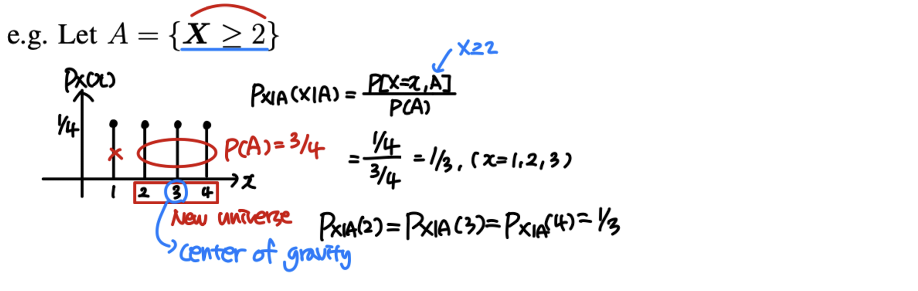
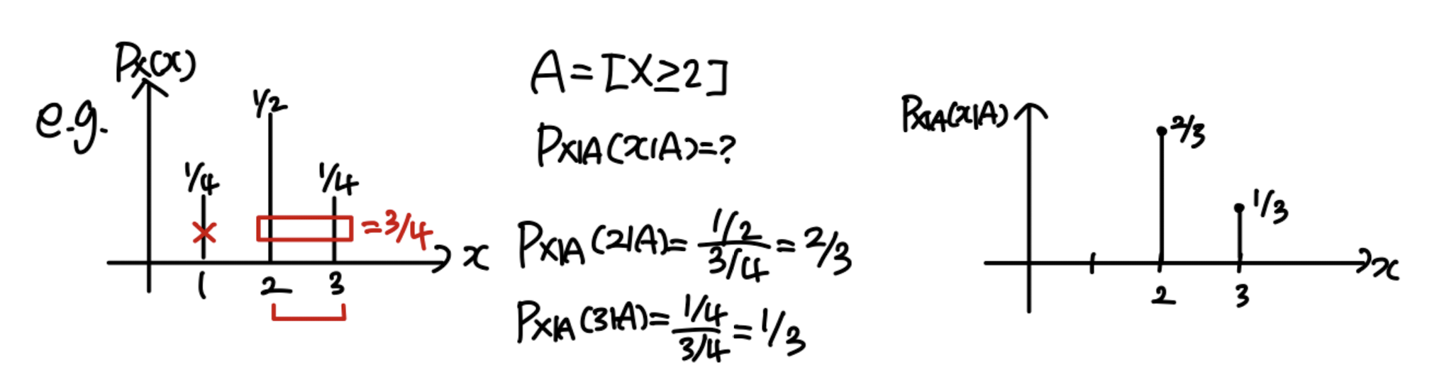
Conditional PMF
P X ∣ A ( x ∣ A ) = P [ X = x ∣ A ] P_{X|A}(x|A)=P[X=x|A] P X ∣ A ( x ∣ A ) = P [ X = x ∣ A ]
E [ X ∣ A ] = ∑ x x ∗ P X ∣ A ( x ∣ A ) E[X|A]=\sum_xx*P_{X|A}(x|A) E [ X ∣ A ] = ∑ x x ∗ P X ∣ A ( x ∣ A )
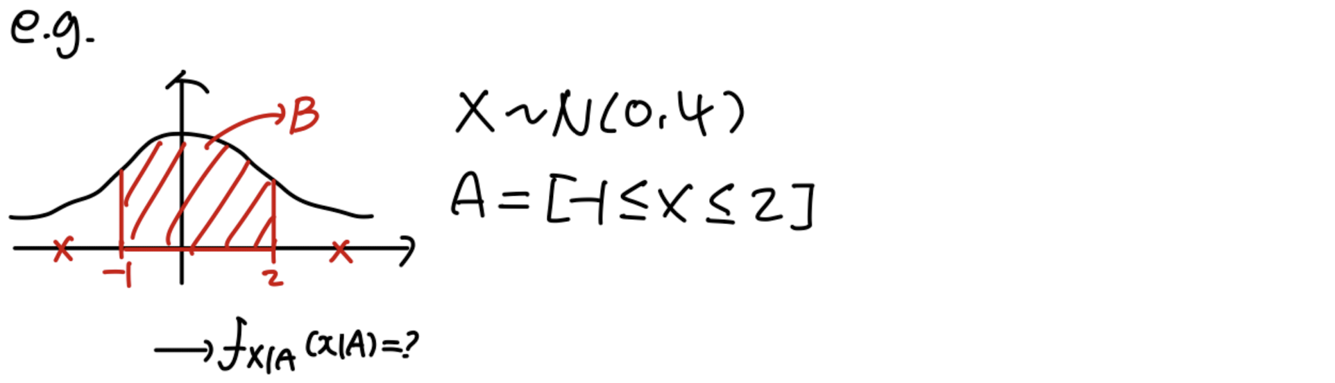
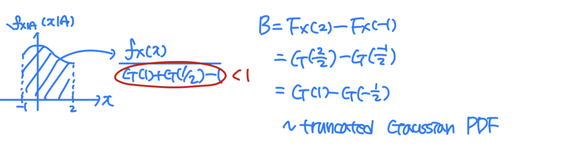
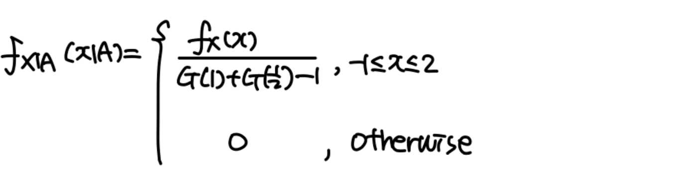
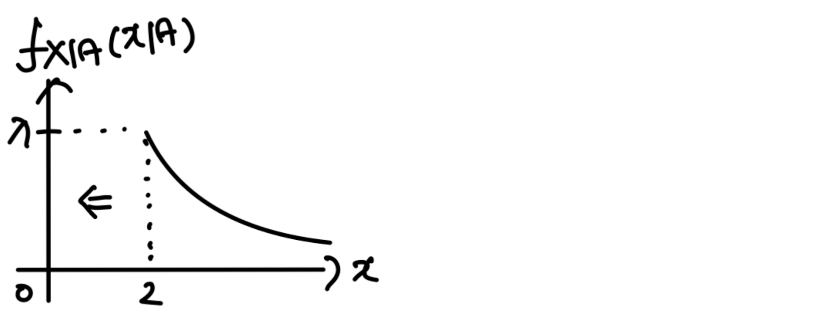
Conditional PDF & CDF
Conditional distribution F X ∣ A ( x ∣ A ) = P [ X ≤ x ∣ A ] F_{X|A}(x|A)=P[X\le x|A] F X ∣ A ( x ∣ A ) = P [ X ≤ x ∣ A ] f X ∣ A ( x ∣ A ) = d d x F X ∣ A ( x ∣ A ) f_{X|A}(x|A)=\frac{d}{dx}F_{X|A}(x|A) f X ∣ A ( x ∣ A ) = d x d F X ∣ A ( x ∣ A ) E [ X ∣ A ] = ∫ − ∞ ∞ x ∗ f X ∣ A ( x ∣ A ) d x E[X|A]=\int^\infin_{-\infin}x*f_{X|A}(x|A)dx E [ X ∣ A ] = ∫ − ∞ ∞ x ∗ f X ∣ A ( x ∣ A ) d x
Total expectation theorem
Recall that P [ B ] = ∑ i = 1 n P [ B ∣ A i ] P [ A i ] P[B] = \sum_{i=1}^nP[B|A_i]P[A_i] P [ B ] = ∑ i = 1 n P [ B ∣ A i ] P [ A i ]
E [ X ] = ∑ i = 1 n E X ∣ A i ( x ∣ A i ) ∗ P [ A i ] E[X]= \sum_{i=1}^n E_{X|A_i}(x|A_i)*P[A_i] E [ X ] = ∑ i = 1 n E X ∣ A i ( x ∣ A i ) ∗ P [ A i ]
For a discrete RV X,
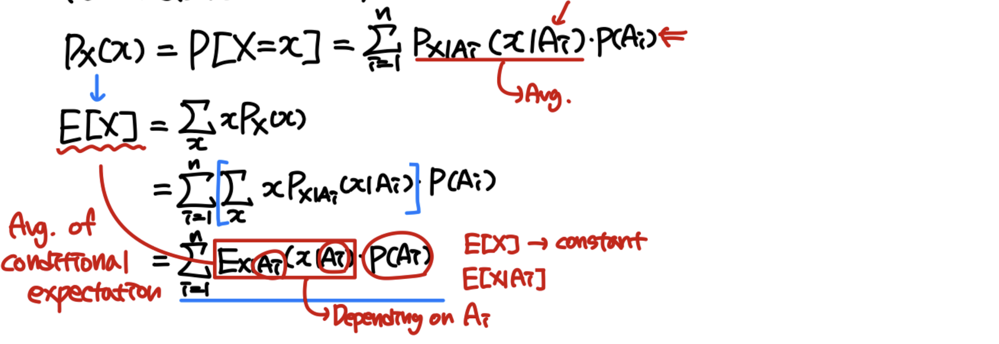
P X ( x ) = P [ X = x ] = ∑ i = 1 n P X ∣ A i ( x ∣ A i ) P [ A i ] P_X(x) = P[X=x]=\sum_{i=1}^nP_{X|A_i}(x|A_i)P[A_i] P X ( x ) = P [ X = x ] = ∑ i = 1 n P X ∣ A i ( x ∣ A i ) P [ A i ] E [ X ] = ∑ x x P X ( x ) E[X]=\sum_xxP_X(x) E [ X ] = ∑ x x P X ( x ) = ∑ i = 1 n ∑ x x P X ∣ A i ( x ∣ A i ) P [ A i ] = \sum_{i=1}^n \sum_xxP_{X|A_i}(x|A_i)P[A_i] = ∑ i = 1 n ∑ x x P X ∣ A i ( x ∣ A i ) P [ A i ] = ∑ i = 1 n E X ∣ A i ( x ∣ A i ) ∗ P [ A i ] = \sum_{i=1}^nE_{X|A_i}(x|A_i)*P[A_i] = ∑ i = 1 n E X ∣ A i ( x ∣ A i ) ∗ P [ A i ]
Similary, for a continuous RV X,
f X ( x ) = ∑ i = 1 n f X ∣ A i ( x ∣ A i ) P [ A i ] f_X(x)=\sum_{i=1}^nf_{X|A_i}(x|A_i)P[A_i] f X ( x ) = ∑ i = 1 n f X ∣ A i ( x ∣ A i ) P [ A i ] E [ X ] = ∫ − ∞ ∞ x f X ( x ) d x E[X]=\int^\infin_{-\infin}xf_X(x)dx E [ X ] = ∫ − ∞ ∞ x f X ( x ) d x = ∑ i = 1 n ∫ − ∞ ∞ x f X ∣ A i ( x ∣ A i ) P [ A i ] d x = \sum_{i=1}^n \int^\infin_{-\infin}xf_{X|A_i}(x|A_i)P[A_i]dx = ∑ i = 1 n ∫ − ∞ ∞ x f X ∣ A i ( x ∣ A i ) P [ A i ] d x = ∑ i = 1 n E X ∣ A i ( x ∣ A i ) ∗ P [ A i ] = \sum_{i=1}^n E_{X|A_i}(x|A_i)*P[A_i] = ∑ i = 1 n E X ∣ A i ( x ∣ A i ) ∗ P [ A i ] ~ Total expectation ~ Expacted value of E X ∣ A i ( x ∣ A i ) E_{X|A_i}(x|A_i) E X ∣ A i ( x ∣ A i )
Memorylessness
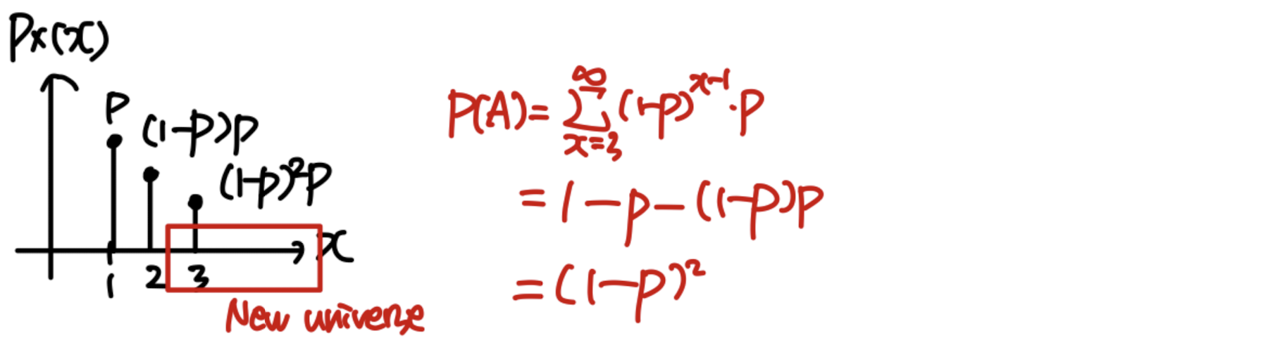
Geometric RV
X ~ # of independent coin tosses until first head
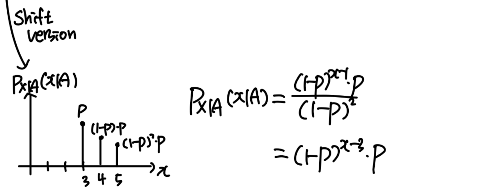
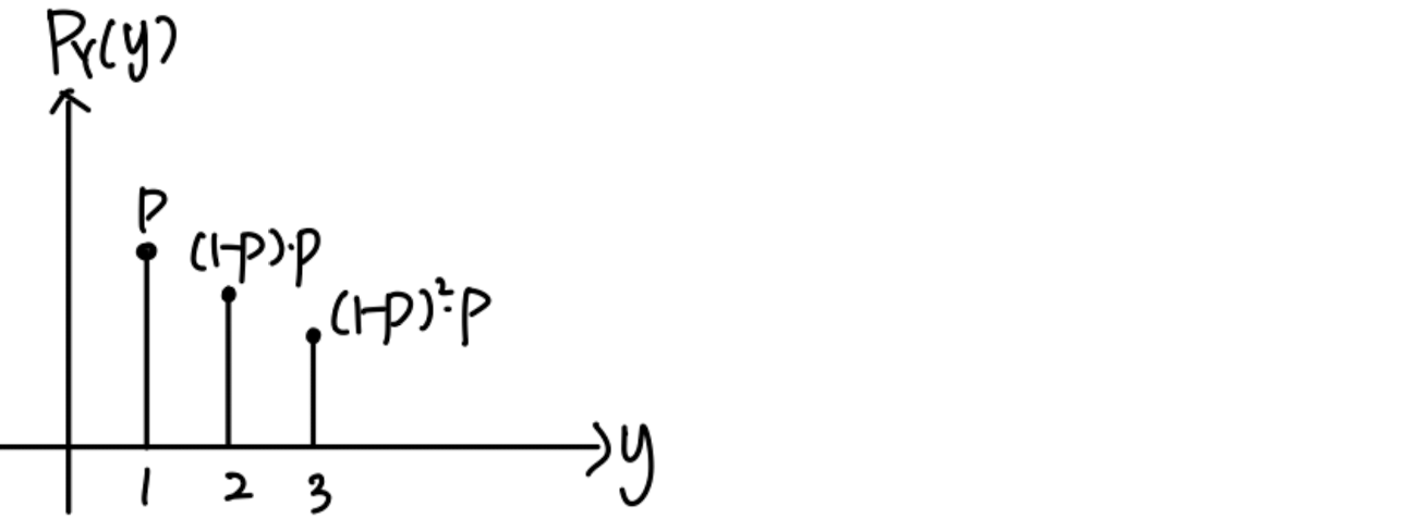
P X ( x ) = ( 1 − p ) x − 1 ∗ p P_X(x) = (1-p)^{x-1}*p P X ( x ) = ( 1 − p ) x − 1 ∗ p A = { X > 2 } A=\{X>2\} A = { X > 2 } P X ∣ A ( x ∣ A ) = P_{X|A}(x|A)= P X ∣ A ( x ∣ A ) = Let Y = X − 2 ( Y > 0 ) Y=X-2 (Y>0) Y = X − 2 ( Y > 0 ) P Y ( y ) = P X ( y ) P_Y(y)=P_X(y) P Y ( y ) = P X ( y )
e.g. P [ X = 5 ∣ X > 2 ] = P [ Y = 3 ∣ X > 2 ] = P [ X = 3 ] P[X=5|X>2]=P[Y=3|X>2]=P[X=3] P [ X = 5 ∣ X > 2 ] = P [ Y = 3 ∣ X > 2 ] = P [ X = 3 ]
Given that X > 2 X > 2 X > 2 Y = X − 2 Y = X − 2 Y = X − 2 X X X
Hence, the geometric random variable is said to be memoryless , because the past has no bearing on its future behavior .
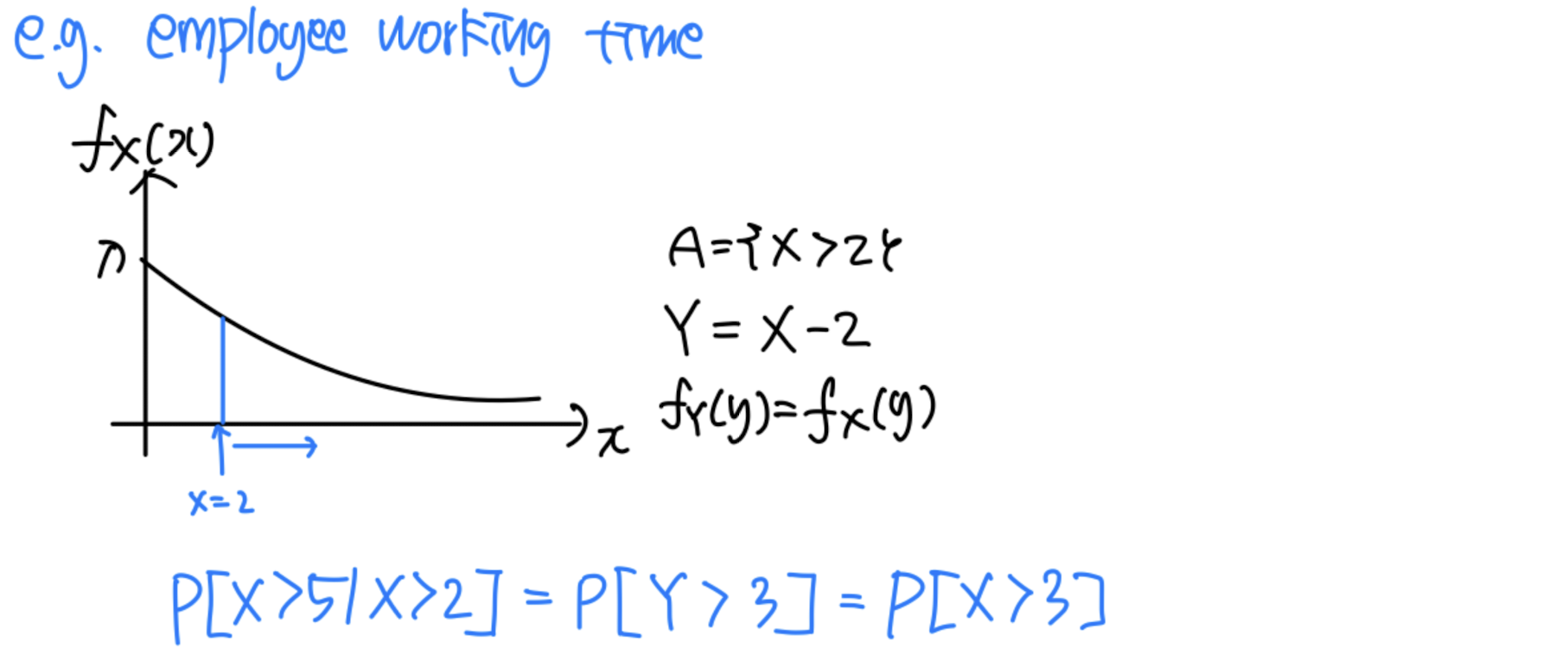
Exponential RV
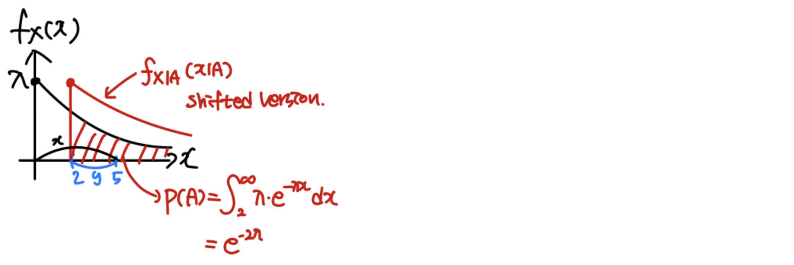
X ~ exponential RV
f X ( x ) = λ e − λ x , x > 0 f_X(x)=\lambda e^{-\lambda x}, x>0 f X ( x ) = λ e − λ x , x > 0 A = { X > 2 } A=\{X>2\} A = { X > 2 } f X ∣ A ( x ∣ A ) = λ e − λ x / e − 2 λ = λ e − λ ( x − 2 ) , x > 2 f_{X|A}(x|A)=\lambda e^{-\lambda x}/e^{-2\lambda}=\lambda e^{-\lambda(x-2)},x>2 f X ∣ A ( x ∣ A ) = λ e − λ x / e − 2 λ = λ e − λ ( x − 2 ) , x > 2 Let Y = X − 2 ( Y > 0 ) Y=X-2 (Y>0) Y = X − 2 ( Y > 0 ) f Y ( y ) = f X ( y ) , y > 0 f_Y(y)=f_X(y), y>0 f Y ( y ) = f X ( y ) , y > 0
e.g. P [ X ≤ 5 ∣ X > 2 ] = P [ Y ≤ 3 ∣ X > 2 ] = P [ X ≤ 3 ] P[X\le5|X>2]=P[Y\le3|X>2]=P[X\le3] P [ X ≤ 5 ∣ X > 2 ] = P [ Y ≤ 3 ∣ X > 2 ] = P [ X ≤ 3 ]
Given that X > 2 X > 2 X > 2 Y = X − 2 Y = X − 2 Y = X − 2 X X X
Hence, the exponential random variable is also memoryless.
Ex_
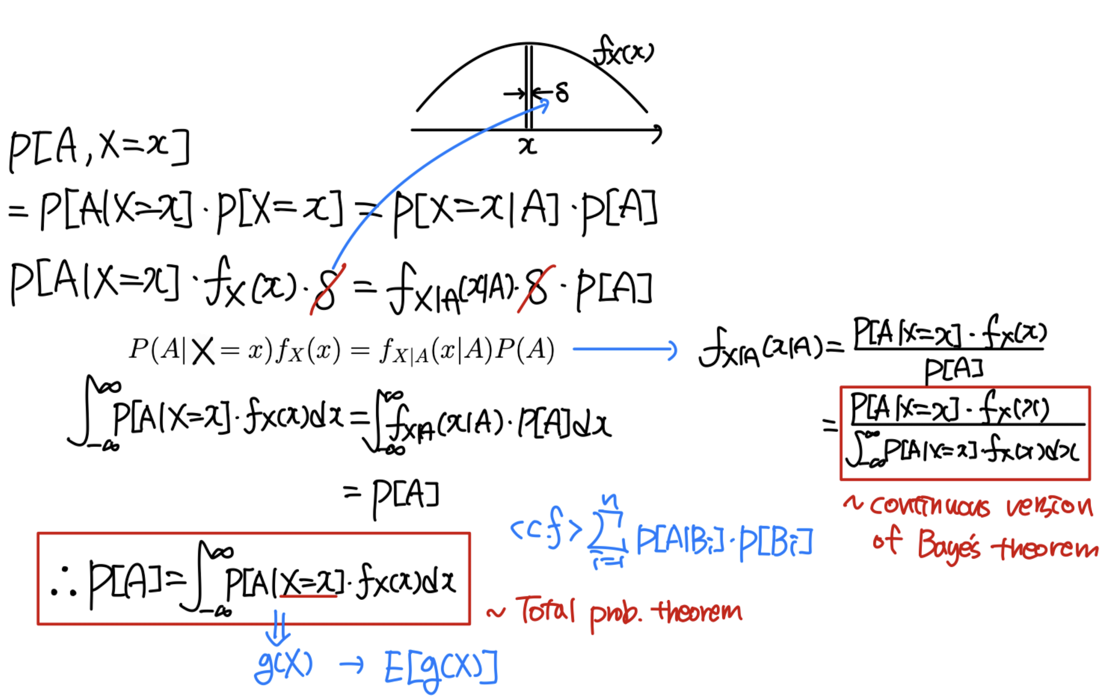
Total probability / Bayes' theorem (continuous ver.)
P [ A ] = ∫ − ∞ ∞ P [ A ∣ X = x ] f X ( x ) P[A] = \int^\infin_{-\infin}P[A|X=x]f_X(x) P [ A ] = ∫ − ∞ ∞ P [ A ∣ X = x ] f X ( x ) f X ( x ) = P [ A ∣ X = x ] f X ( x ) P [ A ] = P [ A ∣ X = x ] f X ( x ) ∫ − ∞ ∞ P [ A ∣ X = x ] f X ( x ) f_X(x)=\frac{P[A|X=x]f_X(x)}{P[A]}=\frac{P[A|X=x]f_X(x)}{\int^\infin_{-\infin}P[A|X=x]f_X(x)} f X ( x ) = P [ A ] P [ A ∣ X = x ] f X ( x ) = ∫ − ∞ ∞ P [ A ∣ X = x ] f X ( x ) P [ A ∣ X = x ] f X ( x )
Coin tossing example
P ( h e a d ) = P P(head)=P P ( h e a d ) = P f P ( p ) f_P(p) f P ( p ) p ∈ [ 0 , 1 ] p\in[0,1] p ∈ [ 0 , 1 ] P ( h e a d ∣ P = x ) = x P(head|P=x)=x P ( h e a d ∣ P = x ) = x P ( h e a d ) = ∫ 0 1 P ( h e a d ∣ P = x ) f P ( x ) d x P(head)=\int^1_0P(head|P=x)f_P(x)dx P ( h e a d ) = ∫ 0 1 P ( h e a d ∣ P = x ) f P ( x ) d x P P P [ 0 , 1 ] [0,1] [ 0 , 1 ] P ( h e a d ) = ∫ 0 1 x ∗ 1 d x = 1 / 2 P(head)=\int^1_0x*1dx=1/2 P ( h e a d ) = ∫ 0 1 x ∗ 1 d x = 1 / 2
HGU 전산전자공학부 이준용 교수님의 23-2 확률변수론 수업을 듣고 작성한 포스트이며, 첨부한 모든 사진은 교수님 수업 PPT의 사진 원본에 필기를 한 수정본입니다.

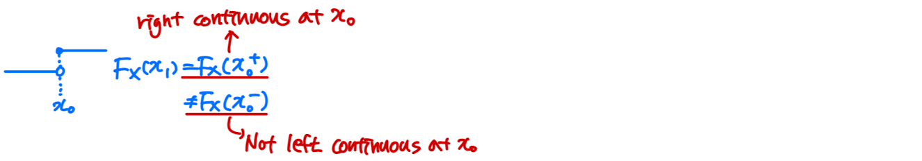
 2. If is descontinuous at , then