
🖥️ Join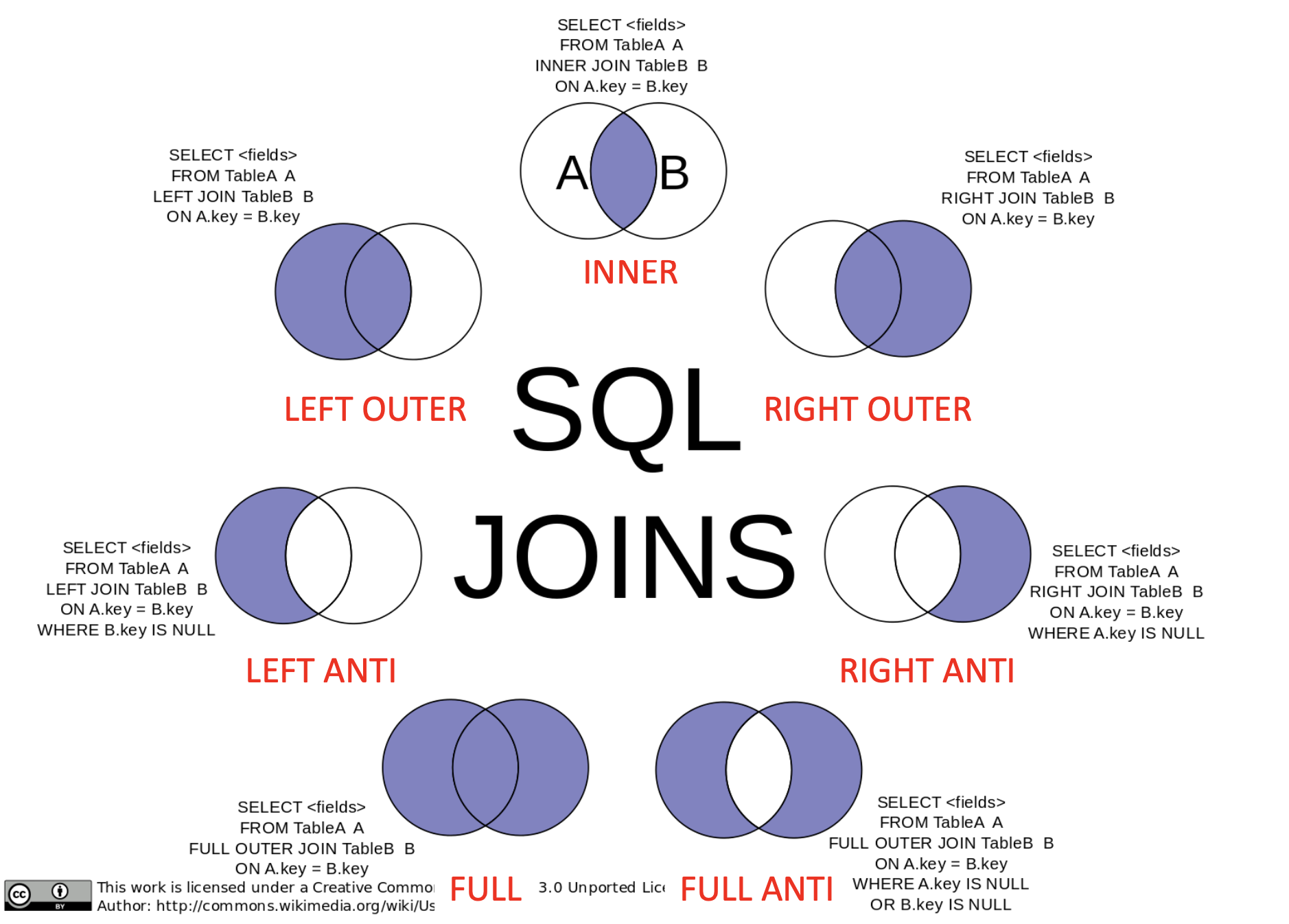
- Join operations take two relations and return another (one) relation
- A join is a Cartesian product that requires tuples in the two relations match
- It also specifies the attributes that are present in the result of the join (project) - Typically used as subquery expressions in the FROM clause
- A join is a Cartesian product that requires tuples in the two relations match
- Join types : Defines how tuples in each relation that do not match any tuples in the other relation are treated
- INNER JOIN : Returns matching data from tables
- OUTER JOIN : Returns matching & some dissimilar data from tables
- Join conditions : Defines which tuples in the two relations match
- NATURAL : Joins two tables based on same attribute name and datatypes
➡️ SELECT * FROM course NATURAL JOIN prereq; - ON < predicate > : Joins two tables based on the column(s) explicitly specified in the ON clause
➡️ SELECT * FROM course
JOIN prereq ON course.course_id = prereq.prereq_id; - USING () : Joins two tables based on common attribute name(s) listed next to USING
➡️ SELECT * FROM course JOIN prereq USING (course_id)
- NATURAL : Joins two tables based on same attribute name and datatypes
Inner join
- Does not preserve nonmatched tuples
- Tables are joined based on common columns mentioned(언급된) in the ON or USING clause
- One can specify the condition with an ON or USING construct
- , Natural join: assumes the join condition to be where same- named columns in both tables match
- Cannot use ON or USING ➡️ Error
- In the result of a natural join, repeated columns are avoided


➡️ more implicit than NATURAL JOIN, less implicit than JOIN ... ON
Outer join
- An extension of the join operation that avoids loss of information
- OUTER JOIN preserves(보존) those tuples that would be lost in a join by creating tuples in the result containing null values
- Computes the JOIN and then adds tuples form one relation that does not match tuples in the other relation to the result of the join
- Returns a set of records that include what an inner join would return
+ other rows for which no corresponding match is found in the other table- Left (outer) join: ”Left” records with no corresponding entry on the “right”


 ➡️ NATURAL LEFT (OUTER) JOIN 순서 기억! 바뀌면 does not work
- Right (outer) join: ”Right” records with no corresponding entry on the “left”


- Full (outer) join: “All” records with no corresponding entry on the other table
➡️ MySQL does NOT support FULL join

- Left (outer) join: ”Left” records with no corresponding entry on the “right”
Natural join
- Some tuples in either or both relations being joined may be lost
- NATURAL JOIN matches tuples with the same values for all common attributes, and retains(유지) only one copy of each common column
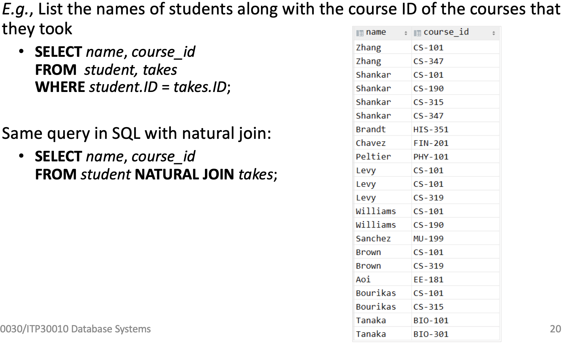
- The FROM clause can have multiple relations combined using natural join:
- SELECT A, A, ... A
FROM r NATURAL JOIN r NATURAL JOIN ... NATURAL JOIN r
WHERE P ;
➡️ Sequantial하게 JOIN
- SELECT A, A, ... A
Caveat(경고) ➡️ 주의해서 사용
E.g., (Incorrect)
SELECT dept_name, course_id, name, title, credits
FROM student NATURAL JOIN takes NATURAL JOIN course;

- Beware(주의) of unrelated attributes with same name getting equated incorrectly
- E.g., List the names of students along with the titles of courses that they have taken
- Correct
SELECT name, title
FROM student NATURAL JOIN takes, course
WHERE takes.course_id = course.course_id;
- Incorrect
SELECT name, title
FROM student NATURAL JOIN takes NATURAL JOIN course;
➡️ This query omits all (student name, course title) pairs where the student takes a course in a department other than the student's own department
- E.g., List the names of students along with the titles of courses that they have taken
Natural Join with USING Clause
- To avoid the danger of equating attributes erroneously, use the USING construct
- USING: allows us to specify exactly which columns should be equated
- E.g.,
SELECT name, title
FROM (student NATURAL JOIN takes) JOIN course USING (course_id)
JOIN ... ON
- The ON condition allows a general predicate over the relations being joined
➡️ Written like a WHERE clause predicate- E.g., SELECT *
FROM student JOIN takes ON student.ID = takes.ID
- The ON condition specifies that a tuple from student matches a tuple from takes if their ID values are equal
- Equivalent to:
SELECT name, course_id
FROM student, takes
WHERE student.ID = takes.ID;
- E.g., SELECT *
INNER JOIN vs. NATURAL JOIN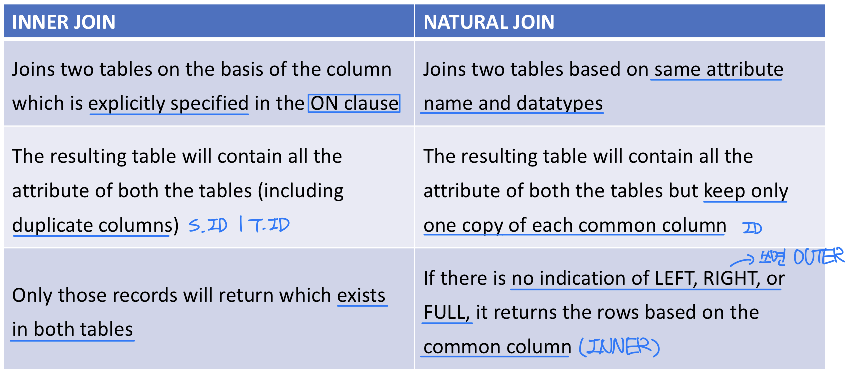
- Inner join
- SELECT * FROM course
(INNER) JOIN prereq ON course.course_id = prereq.prereq_id;
- SELECT * FROM course
- Natural join
- SELECT *
FROM course NATURAL JOIN prereq
ON course.course_id = prereq.prereq_id; ⬅️ NOT VALID!
- SELECT *
Natural Joins Are Often Avoided
- Because:
- ⭐️ Natural joins are not particularly readable (by most SQL coders) and possibly not supported by various tools/libraries
- Natural joins are not informative; you cannot tell what columns are being joined on without referring to the schema
- ⭐️ Your join conditions are invisibly(눈에 띄지않게) vulnerable(취약) to schema changes
- Even if there are multiple natural join columns and one such column is removed from a table, the query will still execute
- But the result may not be correct and this change in behavior will be silent
🖥️ Views
- It is not always desirable for all users to see the entire logical model of data
- E.g., consider a user who needs to know an instructor name and department, but not the salary
➡️ This user only needs to see the following relation (in SQL):- SELECT ID, name, dept_name
FROM instructor
- SELECT ID, name, dept_name
- E.g., consider a user who needs to know an instructor name and department, but not the salary
- View: provides a mechanism to hide certain data from the view of certain users
- A view is a relation defined in terms of stored tables (called base tables) and other views
- Any relation that is not of the conceptual model but is made visible to a user as a "virtual relation" is called a view
- Syntax: CREATE VIEW v AS < query expression >
where < query expression > is any legal SQL expression, and v represents the view name- Once a view is defined, the view name can be used to refer to the virtual relation that the view generates
- View definition is not the same as creating a new relation
- A view definition causes the saving of an expression; the expression is substituted into queries using the view
View Examples
- A view of instructors without their salary:
- CREATE VIEW faculty AS
SELECT ID, name, dept_name
FROM instructor
- CREATE VIEW faculty AS
- Querying on a view is also possible:
- SELECT name
FROM faculty
WHERE dept_name = 'Biology’
- SELECT name
- C.f., find all instructors in the Biology department:
- SELECT name
FROM instructor
WHERE dept_name = 'Biology’
- SELECT name
- DROP VIEW faculty
- The attribute names of a view can be specified explicitly
- CREATE VIEW departments_total_salary(dept_name, total_salary) AS
SELECT dept_name, SUM(salary)
FROM instructor
GROUP BY dept_name;- Since the expression SUM(salary) does not have a name, the attribute name is specified explicitly in the view definition
- CREATE VIEW departments_total_salary(dept_name, total_salary) AS
View Expansion
- View expansion: A way to define the meaning of views defined in terms of other views ➡️ 정의한 view를 또 다른 view definition에 사용할 수 있다
- Let view be defined by an expression that may itself contain uses of view relations
- View expansion of an expression repeats the following replacement step:
repeat
Find any view relation in
Replace the view relation by the expression defining
until no more view relations are present in - As long as the view definitions are not recursive, this loop will terminate
- One view may be used in the expression defining another view
- A view relation v is said to depend directly on a view relation v if v is used in the expression defining v
- A view relation is said to depend on view relation v if either v depends directly to v or there is a path of dependencies from v to v
- A view relation v is said to be recursive if it depends on itself
Example
CREATE VIEW physics_fall_2017 AS
	SELECT course.course_id, sec_id, building, room_number
  	FROM course, section
	WHERE course.course_id = section.course_id
		AND course.dept_name = 'Physics'
  		AND section.semester = 'Fall'
		AND section.year = '2017';

CREATE VIEW physics_fall_2017_watson AS
  	SELECT course_id, room_number
 	FROM physics_fall_2017
  	WHERE building= 'Watson';
➡️ A view is used in another view definition
CREATE VIEW physics_fall_2017_watson AS
  	SELECT course_id, room_number
	FROM physics_fall_2017
	WHERE building= 'Watson';

CREATE VIEW physics_fall_2017_watson AS
	SELECT course_id, room_number
	FROM (
  		SELECT course.course_id, sec_id, building, room_number
		FROM course, section
		WHERE course.course_id = section.course_id
			AND course.dept_name = 'Physics'
  			AND section.semester = 'Fall'
			AND section.year = '2017'
 	)
	WHERE building= 'Watson';
➡️ Both queries are equivalent (view expansion)
Materialized Views
- Two kinds of views
- Virtual: not stored in the database; just a query for constructing the relation ➡️ 시간이 오래 걸릴 수 있다
- Materialized: physically constructed and stored ➡️ like caching
- Materialized view: pre-calculated (materialized) result of a query
- Unlike a simple VIEW the result of a Materialized View is stored somewhere, generally in a table
- Used when:
- Immediate response is needed
- The query where the Materialized View bases on would take to long to produce a result
- Materialized Views must be refreshed occasionally
➡️ 주기적으로 update 필요!
why? original table을 update 했을 때, materialized view는 X
- MySQL does NOT support materialized views ➡️ 개념만
Update via a View
- Add a new tuple to faculty view which we defined earlier
INSERT INTO faculty VALUES ('30765', 'Green', 'Music');- This insertion must be represented by the insertion into the instructor relation
- Must have a value for salary
- This insertion must be represented by the insertion into the instructor relation
- Must have a value for salary
1) Reject the insert(salray not allow NULL), OR
2) Inset the tuple ('30765', 'Green', 'Music', null) into the instructor relation - Some updates cannot be translated uniquely
- E.g., CREATE VIEW instructor_info AS
SELECT ID, name, building
FROM instructor, department
WHERE instructor.dept_name = department.dept_name; - then, INSERT INTO instructor_info
VALUES ('69987', 'White', 'Taylor');
- E.g., CREATE VIEW instructor_info AS
- Issues
- Which department, if multiple departments are in Taylor?
- What if no department is in Taylor?
- On MySQL, an "SQL error (1394): Can not insert into join view without fields list" occurs ➡️ reject
- Example
- CREATE VIEW history_instructors AS
SELECT *
FROM instructor
WHERE dept_name = 'History';
- CREATE VIEW history_instructors AS
- What happens if one inserts ('25566', 'Brown', 'Biology', 100000) into history_instructors?
- INSERT INTO history_instructors
VALUES ('25566', 'Brown', 'Biology', 100000)
- INSERT INTO history_instructors
- Most SQL implementations allow updates only on simple views
- The FROM clause has only one database relation
- The SELECT clause contains only attribute names of the relation, and does not have any expressions, aggregates, or DISTINCT specification
- Any attribute not listed in the SELECT clause can be set to null
➡️ The attribute not shown should allow null - The query does not have a GROUP BY or HAVING clause
🖥️ Window functions
- First introduced to standard SQL in 2003
- Built-in functions that define the relationships between records
- “A window function performs a calculation across a set of table rows that are somehow related to the current row...Behind the scenes, the window function is able to access more than just the current row of the query result” (PostgreSQL)
- ranks, percentiles, sums/averages, row numbers
- For aggregation functions, one can implement moving sums, moving averages, etc.
- One can change the window sizes using the WINDOW_FUNCTION clause
- Cannot be used together with a GROUP BY clause
- Both PARTITION and GROUP BY partition the data and compute some statistics
- Does not reduce the number of records in the result
Window function types
- Aggregate window functions
- SUM(), MAX(), MIN(), AVG(), COUNT(), ...
- Ranking window functions
- RANK(), DENSE_RANK(), PERCENT_RANK(), ROW_NUMBER(), NTILE()
- Value window functions
- LAG(), LEAD(), FIRST_VALUE(), LAST_VALUE(), CUME_DIST(), NTH_VALUE()
Syntax
SELECT WINDOW_FUNCTION ( [ ALL ] expression )
OVER ( [ PARTITION BY partition_list ][ **ORDER BY** order_list] )
FROM table;
- WINDOW_FUNCTION: Specify the name of the window function
- ALL (optional): When you will include ALL it will count all values including duplicates
- C.f., DISTINCT is not supported in window functions
- OVER: Specifies the window clauses for aggregate functions
- PARTITION BY partition_list: Defines the window (set of rows on which window function operates) for window functions
- If PARTITION BY is not specified, grouping will be done on entire table and values will be aggregated accordingly
- ORDER BY order_list: Sorts the rows within each partition
- If ORDER BY is not specified, ORDER BY uses the entire table
- PARTITION BY partition_list: Defines the window (set of rows on which window function operates) for window functions
Examples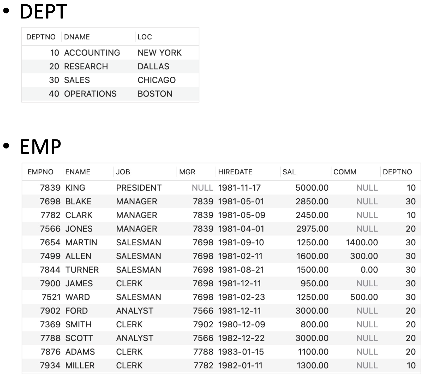
Ranking Examples
- The base query:
- SELECT EMPNO, ENAME, SAL,
SUM(SAL) OVER(ORDER BY SAL
ROWS BETWEEN UNBOUNDED PRECEDING
AND UNBOUNDED FOLLOWING) TOTSAL
FROM EMP;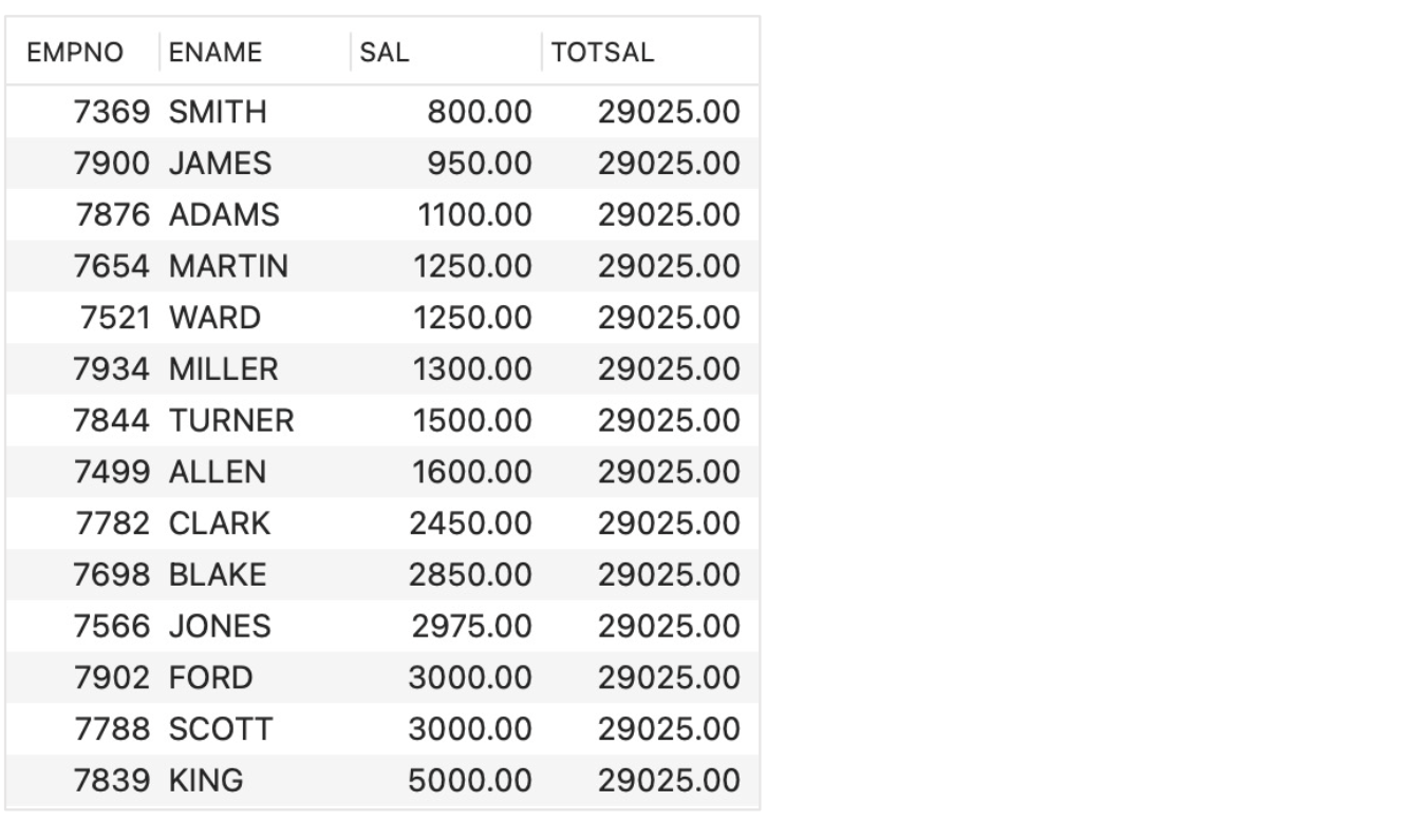
- SELECT EMPNO, ENAME, SAL,
- A cumulative sum:
- SELECT EMPNO, ENAME, SAL,
SUM(SAL) OVER(ORDER BY SAL
ROWS BETWEEN UNBOUNDED PRECEDING
AND CURRENT ROW) TOTSAL
FROM EMP;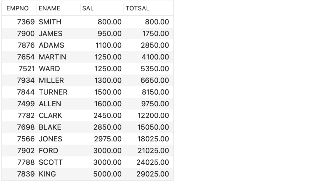
- SELECT EMPNO, ENAME, SAL,
- A table with the total rank and partitioned rank:
- SELECT ENAME, SAL,
RANK() OVER (ORDER BY SAL DESC) ALL_RANK,
RANK() OVER (PARTITION BY JOB ORDER BY SAL DESC) JOB_RANK
FROM EMP;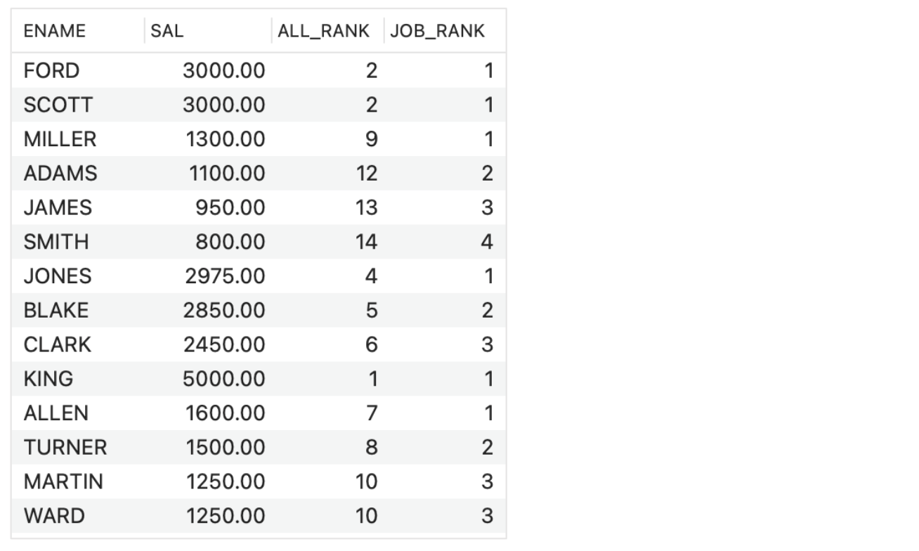
- SELECT ENAME, SAL,
- A table with the total rank and partitioned rank:
- SELECT ENAME, SAL,
RANK() OVER (ORDER BY SAL DESC) ALL_RANK,
DENSE_RANK() OVER (PARTITION BY JOB ORDER BY SAL DESC) JOB_RANK
FROM EMP;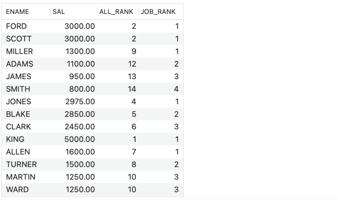
- SELECT ENAME, SAL,
- A table with the total rank and partitioned rank:
- SELECT ROW_NUMBER() OVER (ORDER BY SAL DESC) ROW_NUM,
ENAME, SAL,
RANK() OVER (ORDER BY SAL DESC) ALL_RANK
FROM EMP;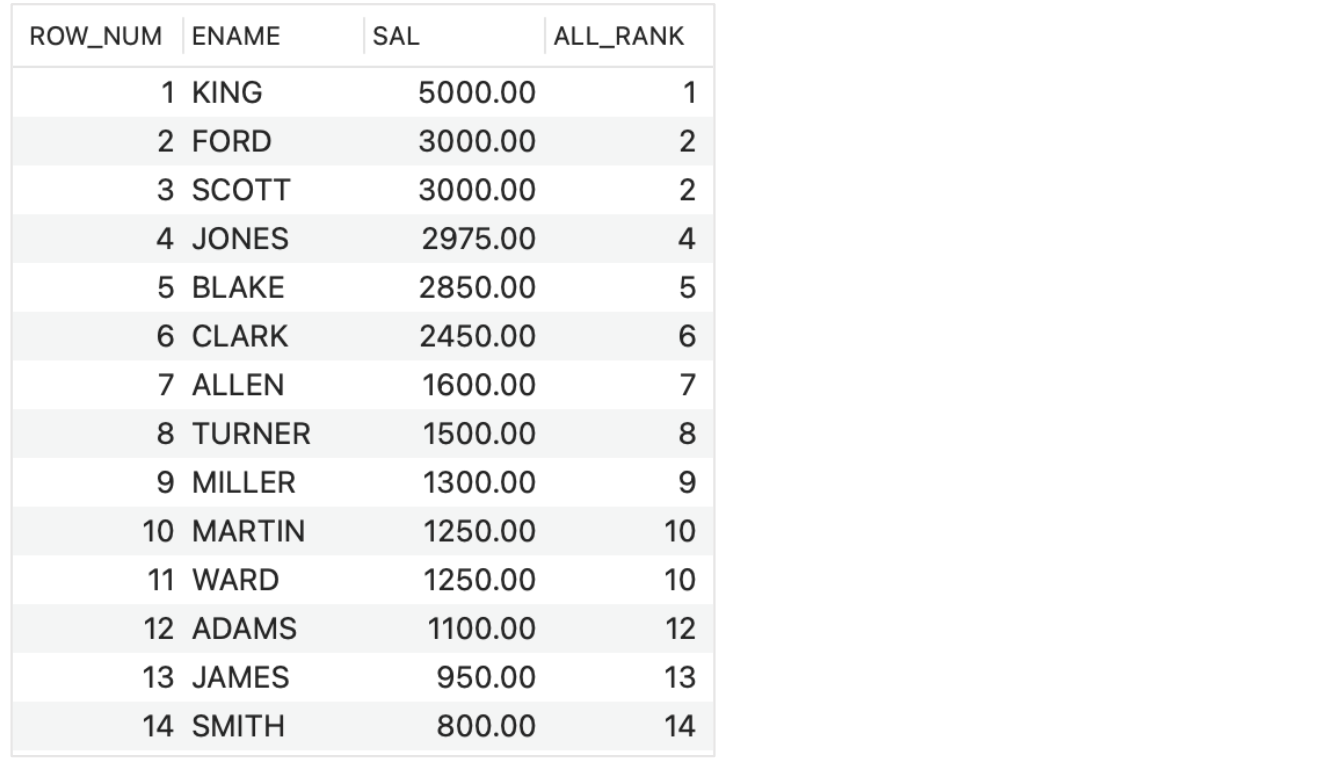
- SELECT ROW_NUMBER() OVER (ORDER BY SAL DESC) ROW_NUM,
Aggregation Eamples
- Average over each job
- SELECT ENAME, SAL, JOB,
AVG(SAL) OVER (PARTITION BY JOB) AS AVG_SAL_JOB
FROM EMP;
- SELECT ENAME, SAL, JOB,
- C.f., Aggregation over groups
- SELECT JOB, AVG(SAL)
FROM EMP
GROUP BY JOB;
- SELECT JOB, AVG(SAL)
- Sum over each manager
- SELECT ENAME, SAL, MGR,
SUM(SAL) OVER (PARTITION BY MGR) SUM_MGR
FROM EMP;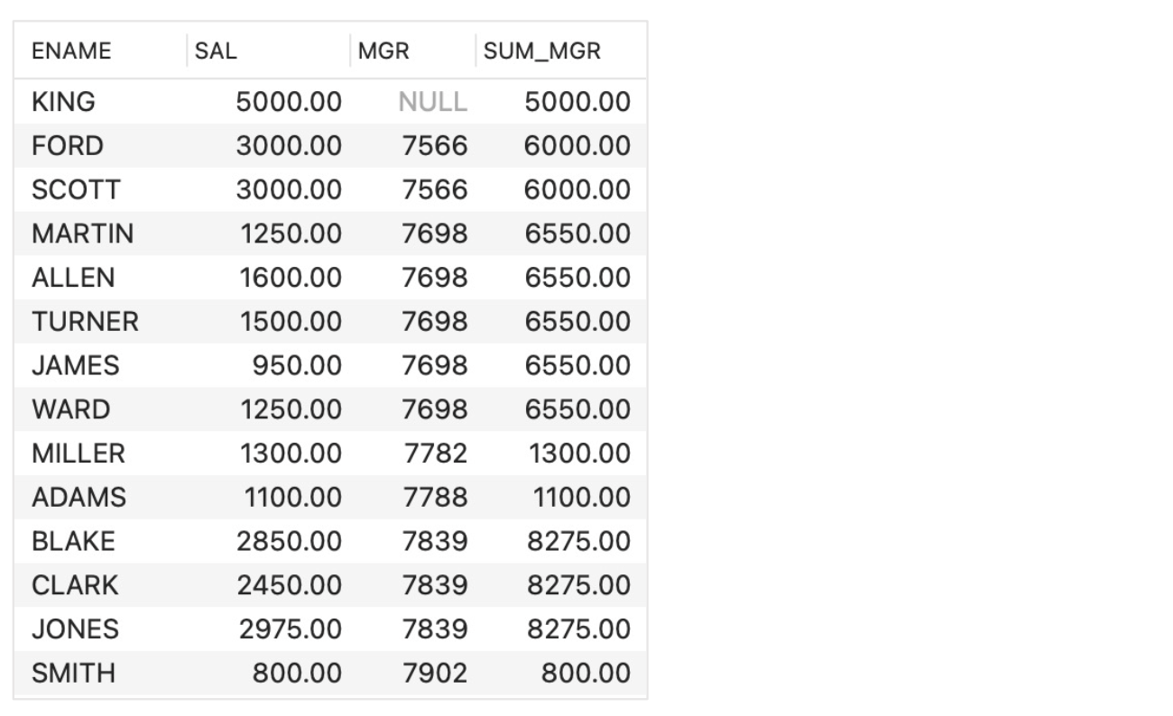
- SELECT ENAME, SAL, MGR,
Nonaggregation Examples
- Rank by salary
- SELECT ENAME, SAL, JOB, HIREDATE,
ROW_NUMBER() OVER (ORDER BY SAL) AS ROW_NUMBER_SAL,
RANK() OVER (ORDER BY SAL) AS RANK_SAL,
DENSE_RANK() OVER (ORDER BY SAL) AS DENSE_RANK_SAL
FROM EMP;
➡️ No PARTITION, consider the entire table as one partition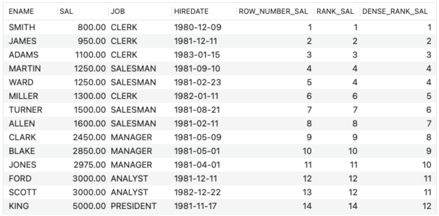
- SELECT ENAME, SAL, JOB, HIREDATE,
- Rank by hiredate
- SELECT ENAME, SAL, JOB, HIREDATE,
ROW_NUMBER() OVER (ORDER BY HIREDATE) AS ROW_NUMBER_HIREDATE,
RANK() OVER (ORDER BY HIREDATE) AS RANK_HIREDATE,
DENSE_RANK() OVER (ORDER BY HIREDATE) AS DENSE_RANK_HIREDATE
FROM EMP;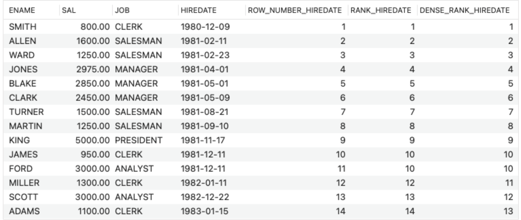
- SELECT ENAME, SAL, JOB, HIREDATE,
- Rank by hiredate within each job
- SELECT ENAME, SAL, JOB, HIREDATE,
RANK() OVER (PARTITION BY JOB ORDER BY HIREDATE DESC) AS RANK_HIREDATE
FROM EMP;
➡️ 1. PARTITION, 2. ORDERING - SELECT ENAME, SAL, JOB, HIREDATE,
RANK() OVER w AS RANK_HIREDATE
FROM EMP
WINDOW w AS (PARTITION BY JOB ORDER BY HIREDATE DESC);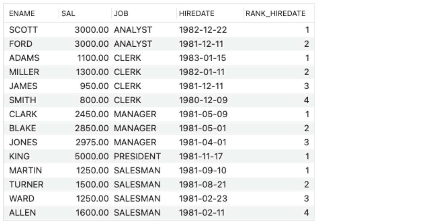
- SELECT ENAME, SAL, JOB, HIREDATE,
- Percentile by salary within each job
- SELECT ENAME, SAL, JOB, HIREDATE,
RANK() OVER (ORDER BY SAL) AS RANK_SAL,
CUME_DIST() OVER (ORDER BY SAL) AS CUME_DIST_SAL,
PERCENT_RANK() OVER (ORDER BY SAL) AS PERCENT_RANK_SAL
FROM EMP; - SELECT ENAME, SAL, JOB, HIREDATE,
RANK() OVER w AS RANK_SAL,
CUME_DIST() OVER w AS CUME_DIST_SAL,
PERCENT_RANK() OVER w AS PERCENT_RANK_SAL
FROM EMP
WINDOW w AS (ORDER BY SAL);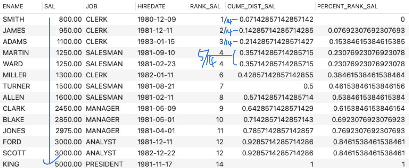
- SELECT ENAME, SAL, JOB, HIREDATE,
Value Window Examples
- First and last records in each partition
- SELECT ID, CITY, ORD_DATE,
FIRST_VALUE(ORD_DATE) OVER(PARTITION BY CITY) AS FIRST_VAL,
LAST_VALUE(ORD_DATE) OVER(PARTITION BY CITY) AS LAST_VAL
FROM ORDERS;
- SELECT ID, CITY, ORD_DATE,
- First and last records in each partition
- SELECT ID, CUSTOMER_NAME, CITY, ORD_AMT, ORD_DATE,
LAG(ORD_DATE,1) OVER(ORDER BY ORD_DATE) AS PREV_ORD_DAT,
LEAD(ORD_DATE,1) OVER(ORDER BY ORD_DATE) AS NEXT_ORD_DAT
FROM ORDERS;
➡️ LAG(ORD_DATE, 1) : before one, LEAD(ORD_DATE, 1) : after one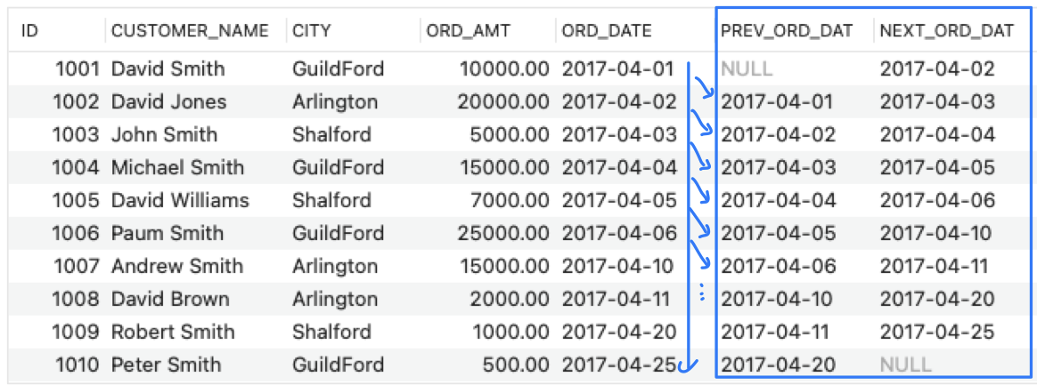
- SELECT ID, CUSTOMER_NAME, CITY, ORD_AMT, ORD_DATE,
- First and last records in each partition
- SELECT ID, CUSTOMER_NAME, CITY, ORD_AMT, ORD_DATE,
LAG(ORD_DATE,2) OVER(ORDER BY ORD_DATE) AS PREV_ORD_DAT,
LEAD(ORD_DATE,2) OVER(ORDER BY ORD_DATE) AS NEXT_ORD_DAT
FROM ORDERS;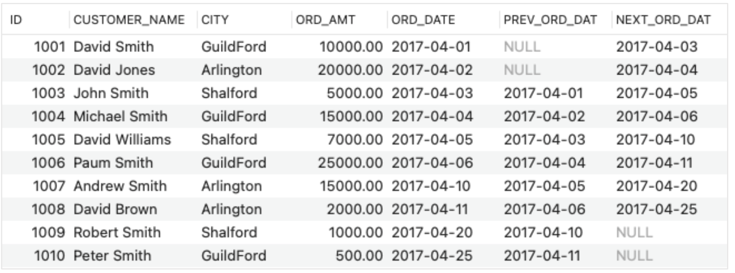
- SELECT ID, CUSTOMER_NAME, CITY, ORD_AMT, ORD_DATE,
Frame Specification
- A frame is a subset of the current partition, and the frame clause specifies how to define the subset
- Frames are determined with respect to the current row
- By defining a frame to be all rows from the partition start to the current row, one can compute running totals for each row
- By defining a frame as extending N rows on either side of the current row, one can compute rolling averages
- ROWS: The frame is defined by beginning and ending row positions (physical window)
- RANGE: The frame is defined by rows within a value range (logical window)
- BETWEEN ... AND ...: Specify both frame endpoints
- UNBOUNDED PRECEDING: The bound is the first partition row
- UNBOUNDED FOLLOWING: The bound is the last partition row
- CURRENT ROW: For ROWS, the bound is the current row; For RANGE, the bound is the peers of the current row
- Frames are determined with respect to the current row
Examples
- Sum over each partition
- SELECT ID, CITY, ORD_AMT, ORD_DATE,
AVG(ORD_AMT) OVER ( PARTITION BY CITY ORDER BY ORD_DATE
ROWS BETWEEN UNBOUNDED PRECEDING ➡️ Begining of the partition
AND UNBOUNDED FOLLOWING ➡️ End of the partition
) AS AVG_AMT
FROM ORDERS;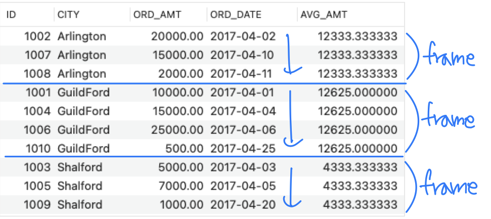
- SELECT ID, CITY, ORD_AMT, ORD_DATE,
- A 2-record moving average
- SELECT ID, CITY, ORD_AMT, ORD_DATE,
AVG(ORD_AMT) OVER ( PARTITION BY CITY ORDER BY ORD_DATE
ROWS BETWEEN 1 PRECEDING
AND 0 FOLLOWING
) AS AVG_AMT
FROM ORDERS; - SELECT ID, CITY, ORD_AMT, ORD_DATE,
AVG(ORD_AMT) OVER ( PARTITION BY CITY ORDER BY ORD_DATE
ROWS BETWEEN 1 PRECEDING
AND CURRENT ROW
) AS AVG_AMT
FROM ORDERS;
➡️ if 0 PRECEDING = CURRENT ROW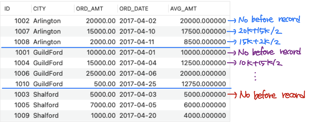
- SELECT ID, CITY, ORD_AMT, ORD_DATE,
- A 3-day moving average
- SELECT ID, ORD_DATE, ORD_AMT,
AVG(ORD_AMT) OVER(ORDER BY ORD_DATE
RANGE BETWEEN INTERVAL 2 DAY PRECEDING
AND CURRENT ROW
) AS AVG_AMT
FROM ORDERS;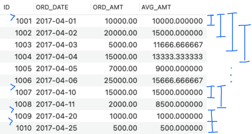
- SELECT ID, ORD_DATE, ORD_AMT,
🖥️ Keys
- Key: An attribute or a set of attributes, which help(s) uniquely identify a tuple of data in a relation
- Why we need keys?
- To force identity of data and
- To ensure integrity of data is maintained
- To establish relationship between relations
➡️ PK - FK : reference integrity
- Why we need keys?

Super key (= UNIQUE)
- Any possible unique identifier
- Any attribute or any set of attributes that can be used to identify tuple of data in a relation; i.e., any of
- Attributes with unique values or
- Combinations of the attributes

Candidate key
- Minimal subset of super key
- If any proper subset of a super key is also a super key, then that (super key) cannot be a candidate key

- If any proper subset of a super key is also a super key, then that (super key) cannot be a candidate key
Primary key
- The candidate key chosen to uniquely identify each row of data in a relation
- No two rows can have the same PK value : No duplicate
- PK value cannot be NULL (every row must have a primary key value)

Alternate key
- The candidate keys that are NOT chosen as PK in a relation

Foreign key
- An attribute in a relation that is used to define its relationship with another relation
- Using foreign key helps in maintaining data integrity for tables in relationship
- Using foreign key helps in maintaining data integrity for tables in relationship
Composite key & Compound key
- Composite key: Any key with more than one attribute
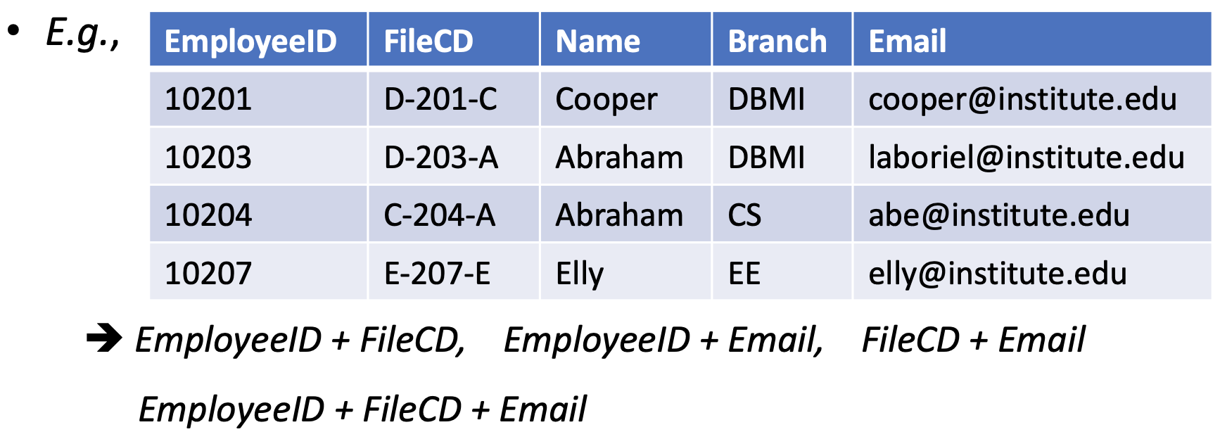
- Compound key: A composite key that has at least one attribute, which is a foreign key
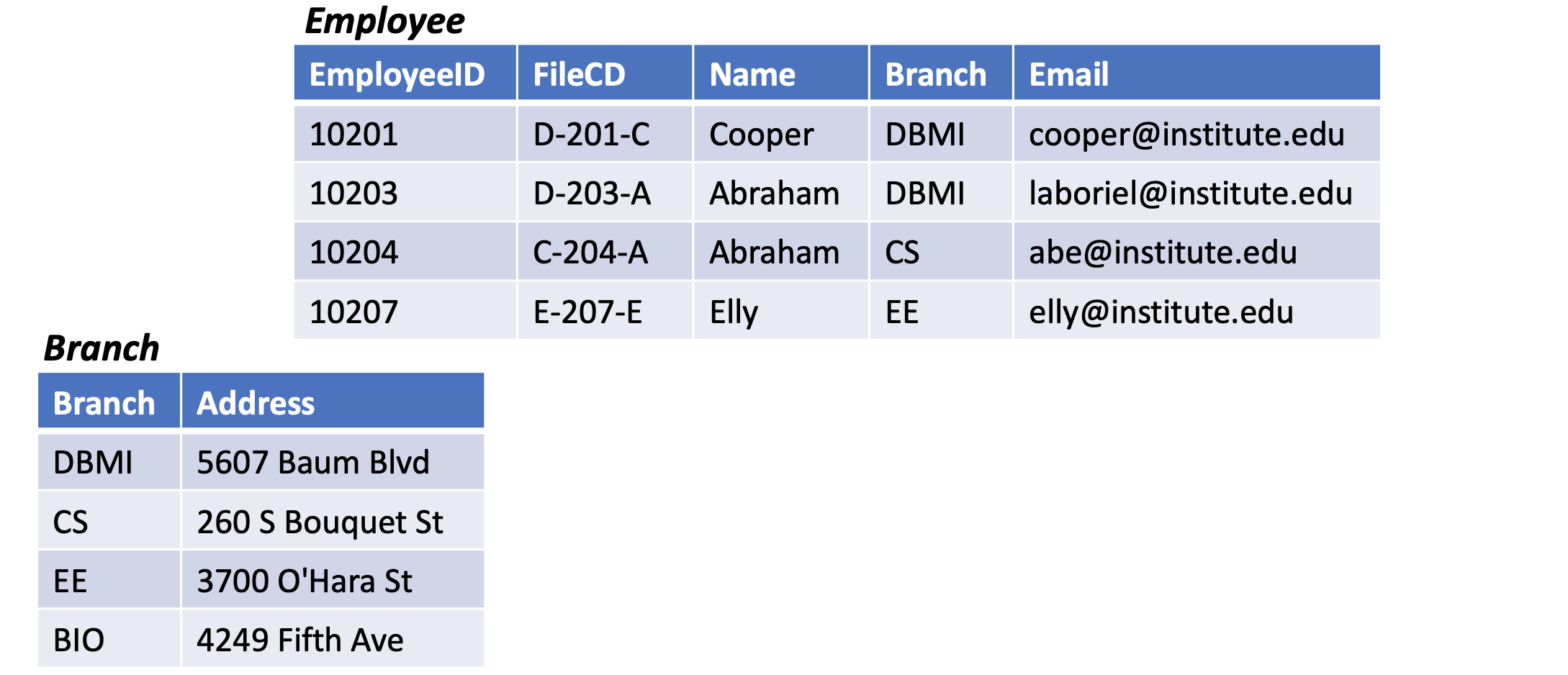
- E.g., Let us assume that we have defined a composite key (FileCD, Branch), it is also a compound key (considering the Branch table)
- E.g., Let us assume that we have defined a composite key (FileCD, Branch), it is also a compound key (considering the Branch table)
- Some composite keys are compound keys
- All compound keys are composite keys
Surrogate key (= Artifical key)
- If a relation has no attribute that can be used as a key, then we create an artificial attribute for this purpose
- It adds no meaning to the data, but serves the sole purpose of identifying tuples uniquely in a table
- ⃝ ⃝ ⃝ ⃝ _ID with auto increment
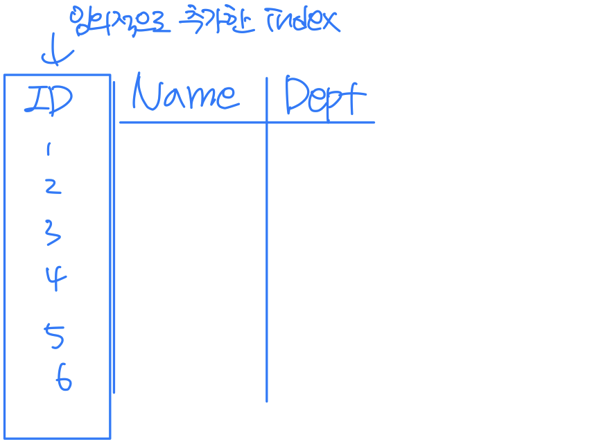
- ⃝ ⃝ ⃝ ⃝ _ID with auto increment
- It adds no meaning to the data, but serves the sole purpose of identifying tuples uniquely in a table
HGU 전산전자공학부 홍참길 교수님의 23-1 Database System 수업을 듣고 작성한 포스트이며, 첨부한 모든 사진은 교수님 수업 PPT의 사진 원본에 필기를 한 수정본입니다.
