TensorBoard

class Net(nn.Module):
    def __init__(self):
        super(Net, self).__init__()
        self.conv1 = nn.Conv2d(1, 6, 5)
        self.pool = nn.MaxPool2d(2, 2)
        self.conv2 = nn.Conv2d(6, 16, 5)
        self.fc1 = nn.Linear(16 * 4 * 4, 120)
        self.fc2 = nn.Linear(120, 84)
        self.fc3 = nn.Linear(84, 10)

    def forward(self, x):
        x = self.pool(F.relu(self.conv1(x)))
        x = self.pool(F.relu(self.conv2(x)))
        x = x.view(-1, 16 * 4 * 4)
        x = F.relu(self.fc1(x))
        x = F.relu(self.fc2(x))
        x = self.fc3(x)
        return x


net = Net()

이전 Classifier 튜토리얼과 유사한 모델 구조를 정의하되, 이미지의 채널이 3개에서 1개로, 크기가 32x32에서 28x28로 변경된 것을 적용할 수 있도록 약간만 수정

1. TensorBoard 설정

from torch.utils.tensorboard import SummaryWriter

# 기본 `log_dir` 은 "runs"이며, 여기서는 더 구체적으로 지정
# runs/fashion_mnist_experiment_1 폴더를 생성합니다.
writer = SummaryWriter('runs/fashion_mnist_experiment_1')

torch.utils 의 tensorboard 를 불러오고,
TensorBoard에 정보를 제공(write)하는 SummaryWriter 를 주요한 객체인 SummaryWriter 를 정의하여 TensorBoard를 설정

2. TensorBoard에 기록하기

# 임의의 학습 이미지를 가져옵니다
dataiter = iter(trainloader)
images, labels = next(dataiter)

# 이미지 그리드를 만듬
img_grid = torchvision.utils.make_grid(images)

# 이미지를 보여줌
matplotlib_imshow(img_grid, one_channel=True)

# tensorboard에 기록
writer.add_image('four_fashion_mnist_images', img_grid)

terator를 이용해 학습 이미지를 가져오고 이미지를 writer.add_image로 TensorBoard에 올림

tensorboard --logdir=runs

cmd에서 실행 후 http://localhost:6006 으로 접속

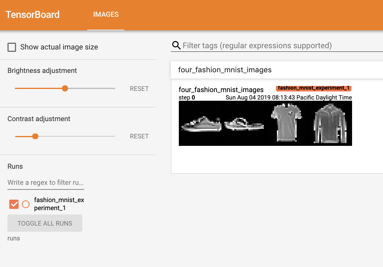
TensorBoard에 올렸던 이미지를 확인할 수 있다

3. TensorBoard를 사용하여 모델 살펴보기(inspect)

writer.add_graph(net, images)
writer.close()

TensorBoard의 강점 중 하나인 복잡한 모델 구조를 시각화하는 기능

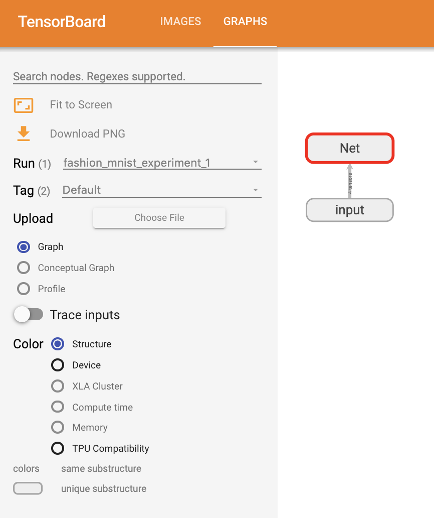
TensorBoard를 새로고침(refresh)하면 《Graphs》 탭을 볼 수 있다.

아래에서 《Net》을 더블클릭하여 펼쳐보면, 모델을 구성하는 개별 연산(operation)들에 대해 자세히 볼 수 있다.

TensorBoard는 이미지 데이터와 같은 고차원 데이터를 저차원 공간에 시각화하는데 매우 편리한 기능들을 제공

4. TensorBoard에 《Projector》 추가하기

# 헬퍼(helper) 함수
def select_n_random(data, labels, n=100):
    '''
    데이터셋에서 n개의 임의의 데이터포인트(datapoint)와 그에 해당하는 라벨을 선택합니다
    '''
    assert len(data) == len(labels)

    perm = torch.randperm(len(data))
    return data[perm][:n], labels[perm][:n]

# 임의의 이미지들과 정답(target) 인덱스를 선택합니다
images, labels = select_n_random(trainset.data, trainset.targets)

# 각 이미지의 분류 라벨(class label)을 가져옵니다
class_labels = [classes[lab] for lab in labels]

# 임베딩(embedding) 내역을 기록합니다
features = images.view(-1, 28 * 28)
writer.add_embedding(features,
                    metadata=class_labels,
                    label_img=images.unsqueeze(1))
writer.close()

add_embedding 메소드(method)를 통해 고차원 데이터의 저차원 표현(representation)을 시각화

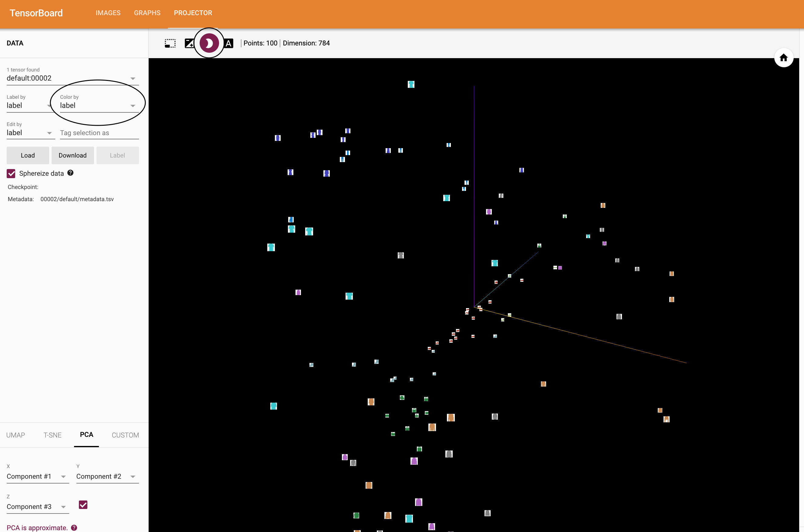
TensorBoard의 《Projector》 - 각각은 784 차원인 - 100개의 이미지가 3차원 공간에 투사(project)된 것을 볼 수 있다.

또한, 이것은 대화식이다: 클릭하고 드래그(drag)하여 3차원으로 투영된 것을 회전할 수 있다.

마지막으로 시각화를 더 편히 볼 수 있는 몇 가지 팁이 있다: 좌측 상단에서 《Color by: label》을 선택하고, 《야간모드(night mode)》를 활성화하면 이미지 배경이 흰색이 되어 더 편하게 볼 수 있다.

5. TensorBoard로 모델 학습 추적하기

TensorBoard에 학습 중 손실을 기록하는 것 대신에 plot_classes_preds 함수를 통해 모델의 예측 결과를 함께 보도록 하겠다.

# 헬퍼 함수

def images_to_probs(net, images):
    '''
    학습된 신경망과 이미지 목록으로부터 예측 결과 및 확률을 생성합니다
    '''
    output = net(images)
    # convert output probabilities to predicted class
    _, preds_tensor = torch.max(output, 1)
    preds = np.squeeze(preds_tensor.numpy())
    return preds, [F.softmax(el, dim=0)[i].item() for i, el in zip(preds, output)]


def plot_classes_preds(net, images, labels):
    '''
    학습된 신경망과 배치로부터 가져온 이미지 / 라벨을 사용하여 matplotlib
    Figure를 생성합니다. 이는 신경망의 예측 결과 / 확률과 함께 정답을 보여주며,
    예측 결과가 맞았는지 여부에 따라 색을 다르게 표시합니다. "images_to_probs"
    함수를 사용합니다.
    '''
    preds, probs = images_to_probs(net, images)
    # 배치에서 이미지를 가져와 예측 결과 / 정답과 함께 표시(plot)합니다
    fig = plt.figure(figsize=(12, 48))
    for idx in np.arange(4):
        ax = fig.add_subplot(1, 4, idx+1, xticks=[], yticks=[])
        matplotlib_imshow(images[idx], one_channel=True)
        ax.set_title("{0}, {1:.1f}%\n(label: {2})".format(
            classes[preds[idx]],
            probs[idx] * 100.0,
            classes[labels[idx]]),
                    color=("green" if preds[idx]==labels[idx].item() else "red"))
    return fig

마지막으로, 이전 튜토리얼과 동일한 모델 학습 코드에서 1000 배치마다 콘솔에 출력하는 대신에 TensorBoard에 결과를 기록하도록 하여 학습을 해보겠다; add_scalar 함수를 사용

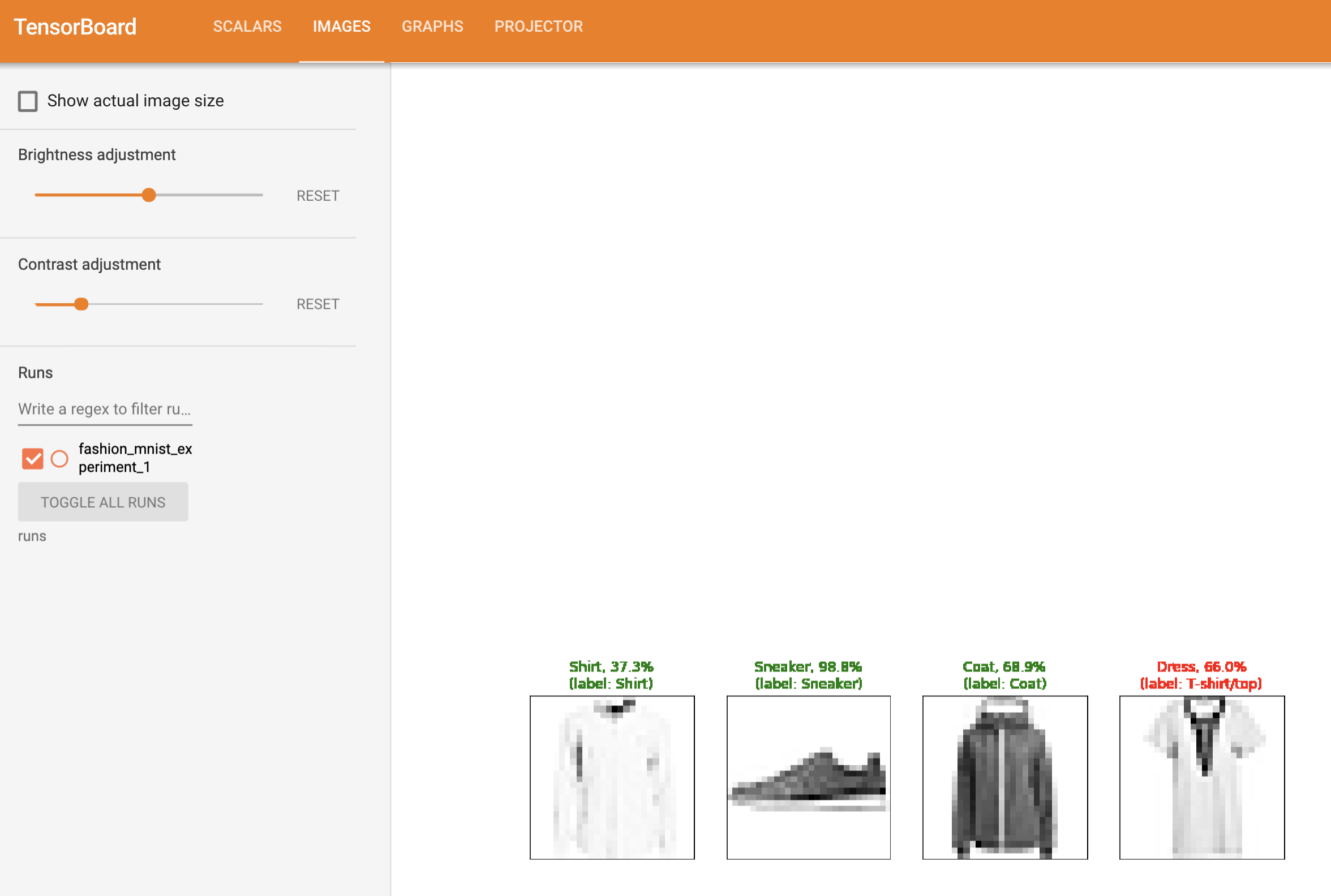
또한, 학습을 진행하면서 배치에 포함된 4개의 이미지에 대한 모델의 예측 결과와 정답을 비교(versus)하여 보여주는 이미지를 생성

running_loss = 0.0
for epoch in range(1):  # 데이터셋을 여러번 반복

    for i, data in enumerate(trainloader, 0):

        # [inputs, labels]의 목록인 data로부터 입력을 받은 후;
        inputs, labels = data

        # 변화도(Gradient) 매개변수를 0으로 만들고
        optimizer.zero_grad()

        # 순전파 + 역전파 + 최적화를 한 후
        outputs = net(inputs)
        loss = criterion(outputs, labels)
        loss.backward()
        optimizer.step()

        running_loss += loss.item()
        if i % 1000 == 999:    # 매 1000 미니배치마다...

            # ...학습 중 손실(running loss)을 기록하고
            writer.add_scalar('training loss',
                            running_loss / 1000,
                            epoch * len(trainloader) + i)

            # ...무작위 미니배치(mini-batch)에 대한 모델의 예측 결과를 보여주도록
            # Matplotlib Figure를 기록합니다
            writer.add_figure('predictions vs. actuals',
                            plot_classes_preds(net, inputs, labels),
                            global_step=epoch * len(trainloader) + i)
            running_loss = 0.0
print('Finished Training')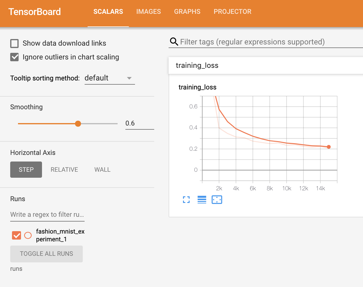

〈Scalars〉 탭에서 15,000번 반복 학습할 때의 손실을 확인

또한, 학습 과정 전반에 걸쳐 임의의 배치에 대한 모델의 예측 결과를 확인할 수 있다. 《Images》 탭에서 스크롤을 내려 《예측 vs. 정답(predictions vs. actuals)》 시각화 부분에서 이 내용을 볼 수 있다;
예를 들어 학습을 단지 3000번 반복하기만 해도, 신뢰도는 높진 않지만, 모델은 셔츠와 운동화(sneakers), 코트와 같은 분류들을 구분할 수 있었다

6. TensorBoard로 학습된 모델 평가하기

이전 튜토리얼에서는 모델이 학습 완료된 후에 각 분류별 정확도(per-class accuracy)를 살펴보았다.

여기서는 TensorBoard를 사용하여 각 분류별 정밀도-재현율(precision-recall) 곡선( 여기 에 좋은 설명이 있습니다)을 그려보겠다.

# 1. 예측 확률을 test_size x num_classes 텐서로 가져옵니다
# 2. 예측 결과를 test_size 텐서로 가져옵니다
# 실행하는데 10초 이하 소요
class_probs = []
class_label = []
with torch.no_grad():
    for data in testloader:
        images, labels = data
        output = net(images)
        class_probs_batch = [F.softmax(el, dim=0) for el in output]

        class_probs.append(class_probs_batch)
        class_label.append(labels)

test_probs = torch.cat([torch.stack(batch) for batch in class_probs])
test_label = torch.cat(class_label)

# 헬퍼 함수
def add_pr_curve_tensorboard(class_index, test_probs, test_label, global_step=0):
    '''
    0부터 9까지의 "class_index"를 가져온 후 해당 정밀도-재현율(precision-recall)
    곡선을 그립니다
    '''
    tensorboard_truth = test_label == class_index
    tensorboard_probs = test_probs[:, class_index]

    writer.add_pr_curve(classes[class_index],
                        tensorboard_truth,
                        tensorboard_probs,
                        global_step=global_step)
    writer.close()

# 모든 정밀도-재현율(precision-recall; pr) 곡선을 그립니다
for i in range(len(classes)):
    add_pr_curve_tensorboard(i, test_probs, test_preds)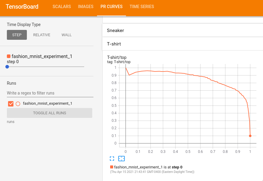

《PR Curves》 탭에서 각 분류별 정밀도-재현율 곡선을 볼 수 있다.
일부 분류는 거의 100%의 《영역이 곡선 아래》에 있고, 다른 분류들은 이 영역이 더 적다

출처 : PyTorch Tutorials https://pytorch.org/tutorials/intermediate/tensorboard_tutorial.html