Summary
It is surprising that Neural ODE can express an differential equation.
I wanna talk about how we can solve the IVP(Initial Value Problem) using Neural Network.
IVP(Initial Value Problem)
IVP is a famous problem in calculus.
h(T)=h(0)+∫0Tdtdh(t)dt
If the h(0) and dtdh(t) is given, then we can calculate the integral and get h(T).
However, computers cannot do the integral operation. We need an algorithm that can make computers calculate the approximate solution of IVP.
Euler Discretization
Given a IVP
h(T)=h(0)+∫0Tdtdh(t)dt
Let's discretize with step size s≈0
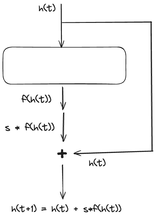
f(h(t))=dtdh(t)
h(t+s)=h(t)+s⋅f(h(t))h(t+2s)=h(t)+s⋅f(h(t+s))...h(T)=h(T−s)+s⋅f(h(T−s))
Given h(t) and f(h(t)), evaluating h(T) is a forward problem.
Given data h(x1),h(x2),...h(xn), getting f(h(t)) is a backword problem.
Euler Discretization with ResNet
It is surprising that Euler Discretization algorithm can be implemented by ResNet. Following image is part of ResNet. We can see the Euler Discretization algorithm can be expressed with ResNet.
Alternative ODE-Solver
Euler Discretization is a very simple(and powerful) algorithm for solving IVP. There are many other ODE-Solver such as Runge-Kutta Method or DOPRI Method. They are all based on Euler Discretization method. It just have more calculation to make it accurate.
In DOPRI Method, it's step size changes depending on the slope of h(t).
Training Neural ODE
We can train the Neural ODE(ResNet) using Normal Backpropagation of ResNet. However, we have a problem.
Assume the total # of steps in DOPRI-Solver is 10,000. If we use Normal Backpropagation Method, we need 10,000 Layers. But this is impossible. Recent research use severel hundreds of layer, and it already requires massive amount of computation for backpropagation.
We need a alternative method for training Neural ODE.
Normal Backpropagation Method
Let's see how it will be trained if we apply normal backpropagation method to Neural ODE.
∂zT∂L is known. zT is the last layer output.
Let's say the step size is h≈0
Let's define at=∂zt∂L.
zt+h=zt+h⋅f(zt)
∂zt∂L=∂zt+h∂L⋅zt∂zt+h
=∂zt+h∂L⋅{1+h⋅∂zt∂f(zt)}
=at+h⋅{1+h⋅∂zt∂f(zt)}
Using the upper equation, we can get the gradient of the layer that outputs zt.
∂θt∂L=∂zt+h∂L⋅∂θt∂zt+h
Then we can derive
∂θt∂L=at+h⋅∂θt∂(zt+h⋅f(zt))=at+h⋅h⋅∂θt∂f(zt)
This means that we need a layer for every steps. This requires huge amount of calculation. We have to think of more better option.
Adjoint Sensitivity Method
Let's go through a simple equation of getting value of z(t+h).
z(t+h)=z(t)+∫tt+hf(z(t′))dt′
This is the start of adjoint method.
Now let's define a(t)=∂z(t)∂L.
a(t)=∂z(t)∂L
=∂z(t+h)∂L⋅∂z(t)∂z(t+h)
=a(t+h)⋅{1+∂z(t)∂∫tt+hf(z(t′))dt′}
Using adjoint method, we can easily calculate the at using dtda(t).
dtda(t)=h→0+limεa(t+ε)−a(t)
=ε→0+limεa(t+ε)−a(t+ε){1+∂z(t)∂∫tt+εf(z(t′))dt′}
Using the following equation,
∫tt+εf(z(t′))dt′=∫tt+ε∂t′∂z(t′)dt′=z(t+ε)−z(t)
We can derive the following equation.
dtda(t)=ε→0+lim−a(t+ε)⋅∂z(t)∂f(z(t))=−a(t)⋅∂z(t)∂f(z(t))
Using dtda(t) and a(T), we can calculate a(t′) for any t′.
We can apply this to the Normal backpropagation method with less layers. We don't need a layer for every step.
∂θt∂L=at+h⋅∂θt∂(zt+h⋅f(zt))=at+h⋅h⋅∂θt∂f(zt)
Summary
I was surprised that we can solve differential equation using ResNet. Machine Learning is integrated into many areas such as physics and mathematics.
