Collapsibility

1. (Non) collapsibility

1.1 An overview

이상적인 무작위 대조군 시험 $(\text{RCT; randomized controlled trial})$에서 표본 크기가 아무리 크더라도 모델에 기저 공변량을 포함할 때 치료받은 집단과 치료받지 않은 집단을 비교하는 추정량이 변한다면 그 모수 측도는 $\text{non-collapsible}$ 성질을 가지고 있습니다. 즉, $\text{confounding}$이 없더라도 결과 변수와 연관되어있는 기저 공변량을 모델에 포함시킬지 여부가 치료 효과의 크기와 관련이 있다는 뜻입니다. 로지스틱 회귀의 오즈비는 $\text{non-collapsible}$이라는 것이 잘 알려져 있습니다. 따라서 조건부 $(\text{conditional})$, 주변부 $(\text{marginal})$ 오즈비 차이는 샘플링 변동성이 아닌 $\text{non-collapsible}$ 성질에 의해 초래됩니다. 참고로 비무작위 연구에서 $\text{non-collapsible}$인 모수를 사용하는 모델을 분석할 때, 모델에 $\text{potential confounders}$을 추가하거나 제거할 경우, 노출 효과 추정값의 변화는 $\text{non-collapsible}$, $\text{confounding}$, 유한 표본 변동 $\text{(finite sample variation)}$이 결합된 결과라는 점에 유의해야 합니다. 이는 공변량이 $\text{confounding}$인지 여부를 결정하기 위해 추정값 변화$\text{(change-in-estimate)}$ 절차를 사용하는 것을 복잡하게 만듭니다.

$\\[30pt]$

1.2 Collapsibility in Contingency Tables

다음은 세 개의 이산 변수 $X,\ Y,\ Z$의 결합 분포를 나타내는 분포표를 통해 $\text{collapsibility}$을 간단히 이해해 보겠습니다.

1. $\ I \times J \times K$ 분할표

2. $X$와 $Y$의 결합 분포를 나타내는 $\ I \times J$ 주변부 분할표

3. $Z$ 수준 내에서 $X$와 $Y$의 결합 분포를 나타내는 조건부 $\ I \times J$ 소(계층) 분할표

계층 $Z$에서 $\text{strictly collapsible}$하다는 것은 "$X$와 $Y$의 연관성 $\text{(association)}$ 측도가 각 계층별에서 일정하고 그 값이 주변부 분할표에서 얻은 값과 동일할 때"를 의미합니다.

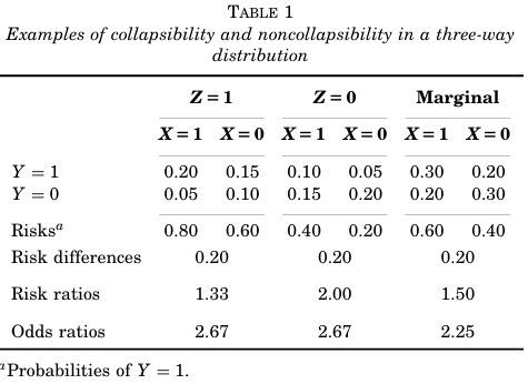
$\text{Table 1}$은 단순한 예제를 제공합니다. $Y = 1$일 $\text{risk difference}$는 $\text{strictly collapsible}$합니다. 그러나 $Y = 1$일 $\text{risk ratio}$은 $\text{strictly collapsible}$하지 않은데, 이는 $\text{risk ratio}$가 계층 $Z$별로 다르기 때문입니다. 또한, $\text{odds ratio}$ 역시 $\text{strictly collapsible}$하지 않은데, 이는 $\text{marginal}$ 값이 일정한 $\text{conditional (stratum-specific)}$값과 같지 않기 때문입니다. 그러므로, $\text{collapsibility}$ 여부는 선택된 $\text{association}$ 척도에 따라 달라집니다.

이제 측정값이 계층별로 일정하지 않지만 특정 $\text{conditional}$ 측정값들의 요약치가 $\text{marginal}$ 측정값과 동일한 경우를 가정해 봅시다. 이를 $Z$에 대해 $\text{collapsible}$하다고 합니다. 예를 들어, $\text{Table 1}$에서 $Z$의 주변부 분포에 표준화된 $\text{risk ratio}$는

$\text{marginal (crude) risk ratio}$와 동일합니다. 따라서 이 측정값은 $\text{Table 1}$에서 $\text{collapsible}$하다고 할 수 있습니다.

$\\[30pt]$

1.3 characteristic collapsibility function

이제 $\text{RCT}$에서 이진 결과에 대한 모델에서의 $\text{(non)collapsibility}$에 대해 수학적으로 논의를 해보겠습니다. 그러나 다음 섹션 2의 논리를 따르면, 지금 다루는 모든 내용은 관찰 연구에서 조건부 및 주변부 인과 모수 간의 비교에도 동일하게 적용됩니다.

만약 $f(\cdot)$가 어떤 링크 함수 (예: $\text{ identity,\ log,\ logit}$)이고, $\nu$는 선형 예측자 척도에서 $X$와 $Y$의 조건부 연관성 $\text{(conditional association)}$으로 정의한다면, $\Pr(Y = 1|X=0,C)$에서 $\Pr(Y = 1|X=1,𝐶)$로 매핑을 조정하는 함수 $g_{\nu}(\cdot)$가 $\text{non-collapsibility}$을 결정하며, 이 함수는 $\text{characteristic collapsibility function (CCF)}$ 라고 정의되며 다음과 같습니다.

$\text{CCF}$의 적용 과정을 간단하게 설명하면 다음과 같다.

1. 먼저 링크 함수를 적용하여 $C$의 함수로서 치료 받지않은 상태 $(X=0)$에서의 확률$(\text{probability})$을 선형 예측기의 척도로 변환.

2. 변환된 선형 예측기 척도에서 $X$와 $Y$의 조건부 연관성 $(\text{conditional association)}\ \nu$ (=조건부 처리 효과) 을 추가

3. 링크 함수의 역함수를 적용하여 $(X=1)$의 확률 척도로 역변환.

Neuhaus와 Jewell (1993)이 보여주었듯이, 효과 측도의 $\text{collapsibility}$ 여부는 본질적으로 이러한 척도의 변화(및 역변화)와 연관되며, 이는 $\text{CCF}$의 성질에 의해 결정됩니다. 이에 대한 자세한 내용은 부록 $A.1$에서 검토하였습니다. 이 논의는 $C = c$가 주어졌을 때 $X$와 $Y$의 조건부 연관성이 $C$에 의존하지 않는다는 (강한) 가정을 전제로 하고 있음을 유의하시기 바랍니다.

다음 두 단계 (즉, 평균화,와 $g_{\nu}$ 적용)는 주변부 효과와 조건부 효과 간의 관계를 정의합니다.

1. $\Pr(Y = 1 | X = 0, C)$는 $\text{CCF}_{g_{\nu}}$를 통해 $\Pr(Y = 1 | X = 1, C)$로 변환합니다.

2. $\Pr(Y = 1 | X = x)$는 $\Pr(Y = 1 | X = x, C)\ (x = 0, 1)$로부터 $C$에 대해 평균값을 계산합니다.

이번에는 $\text{RCT}$에서 이진 결과에 대한 주변부 모델과 조건부 모델을 사용하여 고려해보겠습니다.

주변부 모델은 다음과 같습니다:

기초 공변량 $C$가 주어졌을 때 조건부 모델은 다음과 같습니다:

• $f(\cdot)$: $\text{identity, log, logit}$과 같은 링크 함수

• $X$는 이진 처치

• $\mu(C)$: 기저 공변량 $C$의 함수로, $X$와 독립.

$\Pr(Y = 1|X=x, C)$를 간단히 $p_x(C)$로 쓰면, $p_1(C)$와 $p_0(C)$가 함수 $g_\nu$를 통해 다음과 같이 관련됨을 쉽게 알 수 있습니다:

$\Pr(Y = 1|X=x)$를 간단히 $p_x$로 쓰면, $X$와 $C$의 독립성에 의해

알 수 있습니다. 일반적인 링크 함수의 경우, $\nu > 0$일 때 $g_\nu$는 오목하고 $\nu < 0$일 때 볼록합니다. 이는 $\nu > 0$일 때 $g_\nu''(\cdot)$가 음수이고 $\nu < 0$일 때 양수임을 보임으로써 쉽게 확인할 수 있습니다. 이때 $\text{Jensen}$의 부등식은 $g_\nu$와 $(E)$의 순서를 뒤바꿨을 때 일어나는 현상을 설명합니다: $\text{Jensen}$의 부등식에 따르면, $\text{CCF}$가 선형일 경우에만 이 두 단계의 순서를 변경하여도 값이 일정하며 $(\text{interchangeable})$, $\text{CCF}$가 볼록 $(\text{convex})$한 경우 증가하고 오목 $(\text{concave})$일 경우 감소합니다. 일반적인 링크 함수에서 $\text{CCF}$의 형태는 다음과 같다.

• $g_\nu$가 오목 $\text{(concave)}$하면 $p_1 \leq g_\nu(p_0)$ $(=g_\nu[E\{p_0(C)\}])$
• $g_\nu$가 볼록 $\text{(convex)}$하면 $p_1 \geq g_\nu(p_0)$
• $g_\nu$가 선형 $\text{(linear)}$이면, $p_1 = g_\nu(p_0)$

이는 $\text{non-collapsibility}$ 성질인 "조건부$(\text{conditional})$ 효과와 주변부$(\text{marginal})$ 효과 간의 차이" 뿐 아니라, "조건부 효과에 비해 주변부 효과가 감소하는 이유도 설명합니다". $\text{Figure 2}$는 다양한 링크 함수와 $\nu$ 값에 대한 $\text{CCF}$를 보여줍니다.

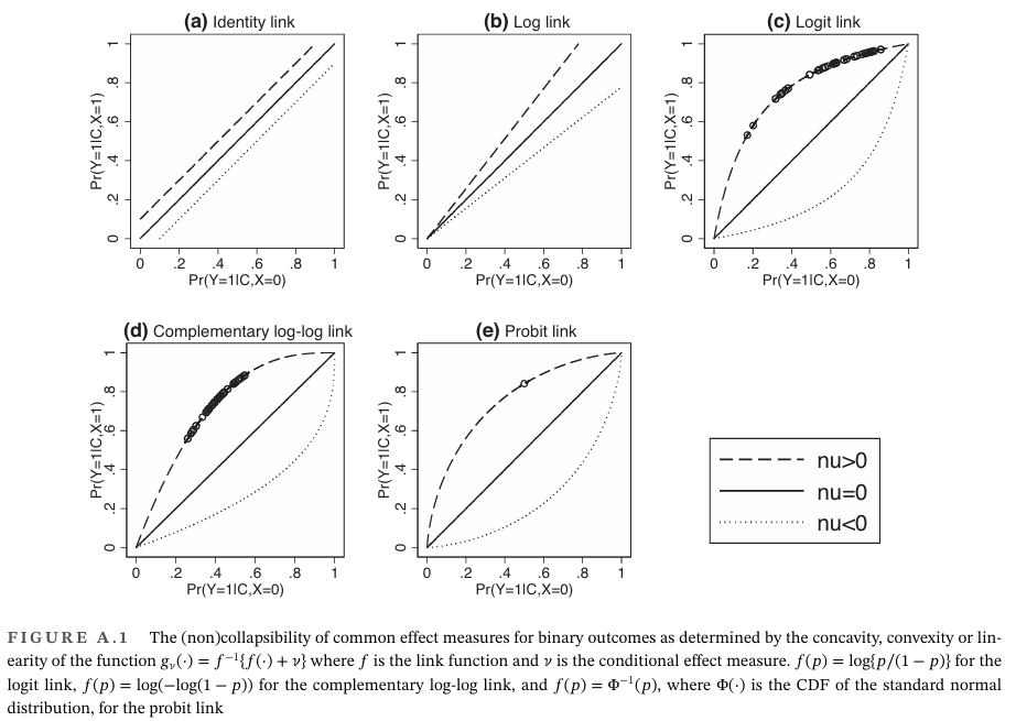
특정 링크 함수를 확인해보면 $\text{identity}$와 $\text{log-link}$ 함수의 경우 $f(p) = p,\ f(p) = \log(p)$으로 $\nu$에 상관없이 $g_\nu(p)$는 $p$에 대해 선형입니다. 그러나

비선형입니다.

따라서 $\beta = f(p_1) - f(p_0)$이며, $f\{g_\nu(p_0)\} - f(p_0) = \nu$입니다. $f$가 증가 함수일 경우(일반적인 링크 함수는 모두 증가 함수), $g_\nu$가 오목일 때 $\beta \leq \nu$, 볼록일 때 $\beta \geq \nu$, 선형일 때는 $\beta = \nu$ 입니다. 이는 주변부 모수 $\beta$가 항상 조건부 모수 $\nu$보다 $\text{null}$에 더 가깝다는 것을 의미합니다 $(|\beta| \leq |\nu|)$. 이는 $\text{non-collapsibility}$가 조건부 효과에 비해 주변부 효과를 "감소"시키는 원인으로 자주 언급되는 이유입니다.

요약하면 선형 $\text{CCF}$는 $\text{identity}$와 같은 선형 링크 함수 뿐만 아니라 $\text{log-link}$ 함수에 의해서도 도출됩니다. 따라서 위험 차이$\text{(risk difference)}$와 위험비$\text{(risk ratio)}$은 $\text{collapsibility}$ 입니다. 오즈비는 $\text{logit link}$ 함수의 비선형성 $(\text{non-linear CCF})$으로 인해 $\text{non-collapsible}$성질을 가집니다. $\text{Figure 2}$에서 볼 수 있듯이, 이항 결과에 흔히 사용되는 대부분의 링크 함수는 비선형 $\text{CCF}$를 내포하며, 따라서 $\text{non-collapsibility}$ 효과 측정값을 초래합니다. 일반적으로 $\text{Figure 2(c) - (e)}$에 있는 세 개의 곡선이 $0$과 $1$에서 만나는 것은 올바른 특성입니다. 이러한 특성은 $(a)$와 $(b)$와 달리, 해당 모델이 확률 범위 $[0,1]$을 벗어나는 값을 예측하지 않도록 방지합니다. 따라서, non-collapsibility는 확률이 $[0,1]$ 범위를 벗어나지 않도록 하는 함수의 굽힘(bending) 현상으로 인해 발생하는 결과이다.

$\text{Figure A.1}$은 일반적으로 $\text{non-collapsibility}$을 초래하는 링크 함수에서도 두 가지 중요한 예외를 보여줍니다.

1. 첫째, 치료 효과가 없을 때 $(\nu = 0)$, $g_{\nu}$는 $f$와 관계없이 항등 $\text{(identity)}$ 함수가 되며, 따라서 모든 효과 측정치는 영가설 하에서 $\text{collapsible}$ 입니다 (이는 영가설 유의성 검정이 $\text{non-collapsibility}$에 의해 영향을 받지 않는 이유입니다).

2. 둘째, $X$가 주어졌을 때 $C$와 $Y$의 조건부 연관이 약해질수록, $\text{Figure A.1}$의 그래프에서 관련된 점들이 점점 더 가까워지고, 비선형성의 정도가 감소합니다. 만약 $X$를 조건로 $C$와 $Y$의 (조건부) 연관이 없다면, 관련 지점은 하나만 남게 되며, 기대값 계산 단계 ($C$에 대한)가 제거되고, 모든 측정치는 $\text{collapsible}$ 됩니다. 우리는 $\text{Figure A.1}$에서 $X$가 주어졌을 때 $C$와 $Y$의 조건부 연관 강도가 점차 약해지는 경우를 나타냈습니다. $(c)$에서는 강한 연관, $(d)$에서는 약한 연관, $(e)$에서는 연관이 없는 경우입니다.
   $\\[30pt]$

1.4 Regression Formulation

위 $1.2$절의 $\text{strictly collapsibility}$ 정의는 회귀 식으로 확장될 수 있습니다. $Y$에 대해 세 가지 회귀 벡터 $W$, $X$, $Z$를 포함한 일반화 선형 모형을 고려해 봅시다:

회귀 분석에서 $\beta$가 $Z$에 대해 $\text{collapsible}$하다고 말하는 것은 $Z$를 생략한 회귀 분석에서 $\beta = \beta^*$가 성립하는 경우를 의미합니다.

$\beta \neq \beta^*$인 경우 $Z$에 대해 $\text{non-collapsible}$합니다. 따라서, 회귀 분석에서 $\beta$가 $Z$에 대해 $\text{collapsible}$하다면, $\beta$가 관심 있는 모수일 경우 $\beta$를 추정하는데 $Z$를 측정할 필요가 없습니니다.

위의 정의는 원래의 교차표 정의를 임의의 변수에 대해 일반화한 것입니다. 그러나 위의 회귀 식의 정의에는 기술적인 문제가 있습니다. 첫 번째(전체) 모델이 정확하다면, 두 번째(축소) 회귀는 주어진 모델 (전체 모델)을 따를 가능성은 낮습니다. 즉, 대부분의 회귀 모델 계열은 $Z$를 제거한 후 닫히지 않습니다. 예를 들어, $Y$가 베르누이 분포이고 $g$가 로짓 링크 함수인 경우, 전체 회귀가 1차 로지스틱 회귀라면 축소된 회귀는 특별한 경우를 제외하고는 1차 로지스틱 모델을 따르지 않습니다. 이 딜레마 (그리고 두 모델 중 어느 것도 정확하게 맞을 가능성이 낮다는 사실)를 해결하는 한 가지 방법은 모델의 모수를 최대가능도 추정량의 비대칭 평균으로 정의하는 것입니다. 이러한 평균은 모델이 정확하지 않더라도 잘 정의되고 해석 가능합니다.

전체 모델이 맞다고 가정할 때, $\delta = 0$은 $\beta$와 $\gamma$가 $Z$에 대해 $\text{collapsibility}$을 가진다는 것을 의미하는 것이 명백할 수 있다. 그러나, $\beta$나 $\delta$가 0이 아닌 경우에는, 설명 변수들의 주변부 독립성 $g$가 항등 $\text{(identity)}$ 이거나 $\text{log-link}$일 경우를 제외하고는 $\beta$가 $Z$에 대해 $\text{collapsibility}$를 가진다는 것을 보장하지 않는다. 반대로, 설명 변수들이 $\text{(association)}$되어 있는 경우에도 $\text{collapsibility}$가 발생할 수 있다. 따라서 $Z$에 대한 $\text{collapsibility}$을 단순한 독립 조건과 동일시하는 것은 일반적으로 올바르지 않지지만, 선형, 로그-선형, 로지스틱 모델과 같은 중요한 특수 사례에서는 유용한 결과를 얻을 수 있습니다.

$\\[40pt]$

2. NOTATION AND FRAMEWORK

섹션 2는 인과 추론 프레임워크 $\text{(causal inference framework)}$에서 잠재적 결과 표기법 $\text{(notation of potential outcomes)}$을 사용하여 오즈비 즉, 로짓 함수의$\text{non-collapsibility}$에 대한 비공식적인 논의를 좀 더 형식적인 수학적 기반으로 전개합니다.

$X$를 이진 노출 또는 치료 변수로 정의하고 ($X=1$은 노출/치료, $X=0$은 비노출/비치료), $Y$는 이진 결과를, $C$는 공변량 집합을 나타냅니다. $C$ 집합은 관찰 연구에서 $\text{potential confounders}$를 포함할 수 있으며, $\text{RCT}$에서는 단순히 기초 공변량을 포함할 수 있습니다. 먼저 중요한 용어의 구분을 설명하겠습니다.

• $\text{associational model vs causal model}$

• $\text{marginal estimands vs conditional estimands}$

• $\text{unadjusted analysis vs adjusted analysis}$

$\\[30pt]$

2.1 Associational and causal models

(A) Associational model

이진 $Y$에 대한 간단한 로지스틱 회귀 모델입니다:

이는 "관찰된 노출군과 비노출군 간" 두 군의 $Y$ 분포를 비교하는 연관 모델 $\text{(associational model)}$입니다.

• $\alpha$: 절편, 비노출군에서의 결과의 로그 오즈 $\text{(log-odds)}$

• $\beta$: 기울기, 노출된 개인과 노출되지 않은 개인 간의 $Y$ 분포를 비교하는 로그 오즈비 $\text{(log-odds ratio)}$.

$\\[30pt]$

(B) causal model

이제 $Y_1$은 한 개인이 노출될 경우의 $\text{potential outcome}$이고, $Y_0$은 이 개인이 노출되지 않을 경우의 해당 $\text{potential outcome}$입니다. 그렇다면, 이진 결과에 대해 다음과 같은 $\text{(saturated)}$ 로지스틱 회귀 모델을 작성할 수 있습니다:

이 모델은 $\text{causal model}$입니다. 왜냐하면, 이는 실제 세계에서의 $Y$와 $X$의 분포를 설명하는 것이 아니라, $X$가 개입된 가상 세계에서의 $Y$의 분포를 설명하기 때문입니다.

• $\phi$: $\text{causal log odds ratio}$, 모두가 노출되었을 때와 모두가 노출되지 않았을 때의 결과를 비교 (현실에 두 결과를 관찰하기는 불가능).

따라서, $\beta$는 관찰된 그룹 간 비교, $\phi$는 개별 비교로 (하나의 결과만 관찰되고 나머지 결과는 잠재 결과)쉽게 이해가능하다. 이상적인 $\text{RCT}$에서는 $\beta = \phi$가 되지만, 관찰 연구에서는 노출과 결과 간의 관계가 $\text{confounded}$되어 $\beta \neq \phi$가 됩니다. 따라서 $\beta = \phi$이 되도록 조정해야 합니다. $\text{counfounding}$ 본문문에서 더 자세히 설명됩니다.

2.2 Marginal and conditional estimands

$\text{conditional associational log-odds ratio}$ $\nu$는

$\text{conditional causal log-odds ratio}$ $\xi$와 같다는 결과를 얻을 수 있습니다.

우리가 언급한 바와 같이, $(1),\ (4)$에서의 $\beta,\ \nu$는 연관 모델에서 $\text{associational parameters}$이고, $(2), (5)$에서의 $\phi,\ \zeta$는 인과 모델에서의 $\text{causal parameters}$입니다. 또 다른 중요한 차이점은 $\beta,\ \phi$는 주변부 추정값 $\text{(marginal estimands)}$인 반면, $\nu,\ \zeta$ 는 조건부 추정값 $\text{(conditional estimands)}$으로, 특히 $C$를 조건부로한 조건부 추정값입니다. 예를 들어, $\zeta$의 해석은 다음과 같습니다:

이는 공변량 수준 $C$에 대한 모집단의 하위 집단에서, 모든 사람의 노출을 $1$로 설정한 것과 $0$으로 설정한 것 사이의 로그 오즈 차이를 의미합니다 (현실에 두 결과를 관찰하기는 불가능). 이는 (모델 $(5)$에 따라) $C$의 값에 대해 일정하다고 가정되지만, 이 가정은 쉽게 완화할 수 있습니다. 모델 $(6)$은 조건부 인과 효과입니다.

반면, 인과 추정값인 $\phi$은 주변부 효과입니다. 이는 참 모집단에서 모든 사람의 노출을 $1$로 설정한 것과 $0$으로 설정한 것 사이의의 로그 오즈 차이입니다.

$\phi$와 $\zeta$ 모두 인과 효과를 가지며, $(10)$의 우변은 $C$의 수준에 관계없이 일정하다고 가정되며, 둘 다 참 모집단의 모수 값이지만, 일반적으로 둘은 같지 않습니다 (둘 다 $\text{confounded}$되지 않음, 모수의 표본 오차는 중요하지 않음). 이는 오즈비가 $\text{non-collapsible}$이기 때문입니다. $\phi =\zeta$가 되는 두 가지 상황은 다음과 같습니다:

1. $\tau = 0$일 때, 즉 공변량 $C$과 결과 $Y$가 노출 $X$이 주어진 조건에서 조건부 독립일 때

2. $\zeta = 0$일 때, 즉 노출 $X$과 결과 $Y$가 공변량 $C$이 주어진 조건에서 조건부 독립일 때 (이 경우 노출 $X$이 결과 $Y$에 미치는 영향이 없으므로 $\phi = 0$도 성립함).

다른 모든 상황에서는 $\phi$가 $\zeta$보다 $0$에 더 가까운 값이 입증되었으며 증명은 $1.3$절에 있습니다.

$\\[30pt]$

2.3 Unadjusted and adjusted analyses

$\text{Unadjusted}$는 종종 $\text{marginal}$과 동의어처럼 사용되며, $\text{adjusted}$는 $\text{conditional}$과 동의어처럼 사용됩니다. 이는 $\text{associational parameters}$만 염두에 둔다면 합리적일 것입니다. 주변부 추정값$\text{(marginal estimands)}$인 $\beta$는 $\text{unadjusted analysis}$ (즉, 회귀 모형에 공변량을 포함하지 않은 분석)으로 추정할 수 있는 반면, 조건부 추정값 $\text{(conditional estimands)}$인 𝜈는 $\text{adjusted analysis}$ (즉, 회귀 모형에 모든 공변량 𝐂를 포함한 분석)으로 추정할 수 있습니다.

그러나 우리는 이를 구별하여, 추정값 $\text{(estimand)}$을 나타낼 때는 $\text{conditional/marginal}$이라는 용어를 사용하고, 분석 $\text{(analysis)}$에서는 $\text{adjusted/unadjusted}$라는 용어를 사용할 것입니다. 이는 다음 섹션에서 논의하겠지만, 공변량 $C$를 조정한 분석으로도 $\text{marginal causal log odds ratio}$인 $\phi$추정값을 얻을 수 있기 때문입니다.

$\\[40pt]$

3 ESTIMATING THE MARGINAL CAUSAL LOG ODDS RATIO

3.1 weight moethd

3.2 ESTIMATING THE MARGINAL CAUSAL LOG ODDS RATIO BY REGRESSION ADJUSTMENT

$\text{RCT}$에서는 $\text{marginal causal log odds ratio}$인 $\phi$를 일관되게 추정하기 위해 $C$를 조정할 필요가 없습니다. $\text{randomization}$은 $\phi=\beta$를 의미하며, 따라서 $\text{unadjusted}$ 분석도 편향 없는 추정이 가능합니다. 그러나 관찰 연구에서는, 혼란 요인$\text{(confounding)}$을 통제하려는 시도로 $C$를 조정할 가능성이 높습니다.

다음 가정이 성립할 때

• $\text{counterfactual consistency}$

• $C$가 주어졌을 때 $\text{conditional exchangeability}$ (가정 $(4)$)

• 모델 $(6)$이 올바르게 지정되었다고 가정

그런 다음 $X,Y,C$에 데이터를 대입하여 $(5)$의 모수를 일관되게 추정했다면 (예; $\text{maximum likelihood}$), 추정량 $\nu$는 $\zeta$의 일치 추정량입니다.

$\text{non-null conditional odds ratio}$은 모델에 공변량을 점점 더 많이 포함시킬수록 크기는 무한대로 커질 수 있습니다 (극단적으로, 노출 외의 모든 결과의 원인을 모델에 포함시킨 경우, $\text{true non-null conditional odds ratio}$는 양의 무한대 또는 음의 무한대까지 커질 수 있습니다.). 따라서 일부는 $\text{marginal odds ratio}$ 또는 공변량 집합의 일부에 대해서만 조건화된 $\text{conditional odds ratio}$가 더 의미 있다고 주장할 수 있습니다.

만약 우리가 관심 있는 추정량이 (조건화된 로지스틱 회귀 모델을 적합시킨) 조건부 인과 로그 오즈비 $\zeta$가 아닌 주변부 인과 로그 오즈비 $\phi$에 관심이 있다면 (Zhang, 2008)의 방법을 이용해 쉽게 추정합니다. 또한 Stata와 R의 margins 명령어는 아래에 설명된 단계를 수행합니다.

---

이중 기대값 규칙, $E(A) = E\{E(A|B)\}$에 따르면, 다음과 같습니다.

여기서 $f_{C}(c)$는 $C$에 대한 확률 밀도 함수 $\text{(probability density function)}$입니다. 모델 $(5)$의 모수 추정량을 통해 $\Pr(Y_x=1|C=c)$의 일치 추정량을 얻을 수 있습니다 (우리의 가정에 따르면 이를 모델 $(6)$의 모수와 동일시할 수 있음):

여기서 $\text{expit}(𝑧) = \frac{\exp(𝑧)}{1 + \exp(𝑧)}$입니다.

이를 $(11)$에 대입하고 $C$의 경험적 분포를 $f_C(c)$의 비모수 추정치 $\text{(nonparametric estimator)}$로 사용할 수 있다. 이는 다음 추정량으로 이어집니다:

여기서 $C_i$는 연구에서 관찰된 개별 $i$의 공변량 값입니다 $(i=1,\ldots,n)$

마지막으로, $x=1$과 $x=0$에 대해 이를 평가하고 두 결과 오즈의 로그 비를 계산하면, $\text{covariate-adjusted estimator}$인 $\phi$를 얻을 수 있습니다:

우리는 이것이 $\text{covariate-adjusted estimator of the marginal causal log odds ratio}$의 추정량임을 강조합니다. 만약 $\gamma \neq 0$라면, $\hat{\phi}^{C-A}$는 $\text{unadjusted estimator}$보다 점근적으로 더 효율적 $\text{(asymptotically more efficient)}$입니다. 따라서 공변량 조정 $\text{(covariate-adjustment)}$은 $\text{confounding}$이 없는 경우에도 유용합니다. 이런 상황에서는 $\text{unadjusted estimator}$은 일관성은 있지만 효율적이지는 않습니다.

$\hat{\phi}^U$를 $\text{RCT}$에서 $\text{unadjusted analysis}$을 통해 얻은 $\phi$의 일반적인 최대가능도추정치 $\text{(MLE)}$라고 하자. 즉, $\hat{\phi}^U=\hat{\beta}$이며, 여기서$\hat{\beta}$는 $\beta$의 일반적인 최대가능도추정치 $\text{(MLE)}$이다. $\mathbb{AV}$는 점근 분산 $\text{(asymptotic variance)}$을 나타내며, 모든 관련 모델이 올바르게 지정되었고 (4)가 성립한다고 가정하자. 앞서 언급했듯이,

이는

를 의미하지만,

도 성립합니다. 즉, "사과와 오렌지"가 아닌 "사과와 사과"를 비교하자마자, 공변량 조정이 로지스틱 회귀에서 효율성을 실제로 증가시킨다는 것을 확인할 수 있습니다(Moore & van der Laan, 2009).

다시 말해, $\hat{\phi}^{C-A}$는 $\text{marginal causal log odds ratio}$에 대한 공변량 조정 추정량임을 감안할 때, $\text{conditional}$와 $\text{adjusted}$는 상호 교환적으로 사용해서는 안 된다는 점을 보여줍니다.

$\hat{\phi}^{C-A}$의 통계적 근사 추론은 델타 방법(delta method)을 통해 가능하며, 이는 추론에서 난수 사용을 반대하는 사람들에게 선호되는 옵션입니다. 그러나 비모수 부트스트랩 $\text{(non-parametric bootstrap)}$은 보통 더 나은 성능을 보이며, 구현하기 더 쉽고, 많은 상황에서 수용 가능한 계산 비용으로 실행할 수 있습니다.

---

• References

1. Greenland, S., Robins, J. M., & Pearl, J. (1999). Confounding and collapsibility in causal inference. Statistical Science, 14,29–46. 번역본

2. Daniel R, Zhang J, Farewell D. Making apples from oranges: comparing noncollapsible effect estimators and their standard errors after adjustment for different covariate sets. Biom J 2021; 63(3): 528–557. 번역본