Confounding and noncollapsibility

1. CONFOUNDING AND NONCOLLAPSIBILITY

1) The Divergence

"효과 추정에서 편향의 의미인 $\text{confounding}$ 개념"과 "$\text{non-collapsibility}$ 개념"을 많은 통계학 문헌에서 구분하고 있지 않습니다. 예를 들어, $Y$에 대해 세 가지 회귀 벡터 $W$, $X$, $Z$를 포함한 일반화 선형 모형을 고려해 봅시다:

회귀 분석에서 $\beta$가 $Z$에 대해 $\text{collapsible}$하다는 것은 $Z$를 생략하더라고 $\beta = \beta^*$가 성립하는 경우를 의미합니다.

$(13)$과 $(14)$에서 $\beta \neq \beta^*$일 때 $Z$의 요소를 $\text{confounders}$로 정의합니다. 그러므로, $\beta = \beta^*$인 경우에는 $Z$를 $\text{non-confounders}$입니다.

그럼에도 불구하고, $\text{confounding}$ 개념"과 "$\text{non-collapsibility}$개념"은 동일하지 않습니다: $\text{confounding}$은 $\text{non-collapsibility}$ 여부와 상관없이 발생할 수 있으며, $\text{non-collapsibility}$ 역시 $\text{confounding}$ 여부와 상관없이 발생할 수 있습니다. 수학적으로 동일한 결론에 다른 용어를 사용한 저자들은 $\text{non-collapsibility}$을 $\text{bias}$라 부르고, $\text{confounding}$을 $\text{covariate imbalance}$라고 불렀습니다.

(A) $\text{non-collapsibility without confounding}$

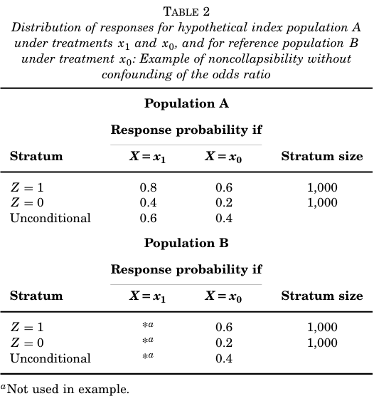
$\text{Table 2}$는 "가상의 목표 모집단 $A$에서 $x_1$ 이거나 $x_0$ 처치 하의 반응변수 분포"와 "가상의 참조 모집단 $B$에서 $x_0$ 처치 하의 반응변수 분포"를 보여준다. $A$는 $x_1$ 처치를, $B$는 $x_0$ 처치를 받았다고 가정하고, "$x_0$ 대신 $x_1$을 받았을 때 $A$에 미친 효과를 추정"하고자 한다. 만약 반응변수의 오즈를 결과 모수 $\mu$로 사용하면,

이 된다. 따라서 오즈비에 대한 $\text{confounding}$은 존재하지 않는다.

이다. 그럼에도 불구하고, 공변량 $Z$는 $A$와 $B$에서 반응변수와 $\text{association}$ 되어 있습니다. 게다가, 오즈비는 $\text{collapsible}$하지 않습니다: $Z$의 수준별로 보면, $x_1$ 처치 하의 모집단 $A$를 $x_0$ 처치 하의 모집단 $A$ 또는 $B$와 비교한 오즈비는

로 $\text{unconditional (crude)}$ 오즈비 2.25보다 높습니다.

이 결과는 효과 척도로서 오즈비의 독특한 성질을 보여줍니다. 처치 $x_1$ (참조 처치 $x_0$ 대비)은 모집단 $A$에서 반응변수의 오즈를 125% 증가시키지만, $Z$의 각 계층 내에서는 반응변수의 오즈를 167% 증가시킵니다. 만약 $Z$가 처치와 $\text{conditional}$로 반응변수와 $\text{association}$되어 있지만, $\text{unconditional}$으로 반응변수와 $\text{association}$되지 않는 경우, 계층별 오즈비는 $\text{unconditional}$ 오즈비가 1이 아닌 경우 더 1에서 멀어지게 됩니다. 이러한 현상은 종종 $\text{unconditional}$ 오즈비의 $\text{bias}$로 해석되지만, 사실 $\text{unconditional}$ 효과를 계층별 또는 개별 효과의 추정치로 잘못 해석하지 않는다면 $\text{bias}$는 존재하지 않습니다.

(B) $\text{confounding without non-collapsibility}$

전체 효과에 대한 오즈비가 $\text{collapsible}$하면서도 $\text{confounded}$한 수치적 예를 생성하려면, $\text{Table 2}$를 약간만 수정하면 된다. 즉, 모집단 $B$에서 $Z = 0$인 층의 크기를 $1,500$으로 변경한다. 이 변경으로 인해 모집단 $B$에서 $Z = 1$의 비율이 0.5에서 0.4로 감소하며, 처치 $x_0$ 하의 모집단 $B$에서의 $\text{unconditional}$ 반응변수의 확률은

이 되고, 처치 $x_0$ 하의 모집단 $B$에서의 $\text{unconditional}$ 반응변수의 오즈 $\mu_{B0}$는

가 된다. 따라서

이며, 결과적으로 오즈비의 $\text{confounding}$이 발생합니다. 모집단 $A$에서 $x_1$이 오즈에 미친 참 효과 $\mu_{A1}/\mu_{A0}$는 이전과 같이 2.25이지만, 이는 $\text{unconditional}$ 오즈비 $\mu_{A1}/\mu_{B0} = 1.50/0.5625 = 2.67$보다 작습니다. 그럼에도 불구하고, 이 $\text{unconditional}$ 오즈비는 계층별 오즈비와 동일하다.

$\\[30pt]$

2) Conditions for Equivalence

$\text{Table 2}$의 예시에서 $\mu$가 결과의 오즈를 나타낼 때, $\mu_{A0}=\mu_{B0}$임을 보여줍니다 $(\text{no confounding})$. 심지어 오즈비가 $\text{confounders}$에 대해 $\text{non-collapsibility}$인 경우에도 해당됩니다. 반대로 수정된 예에서는, 오즈비가 $\text{collapsible}$한 경우에도 $\mu_{A0} \neq \mu_{B0}$가 될 수 있음을 보여줍니다.

$\text{non-confounding}$과 $\text{collapsibility}$사이의 차이에 대한 확률적 설명은 $Z$가 치료와 $\text{unconditional}$로 $\text{unassociated}$하고 충분히 제어되는 경우 $\mu_{A0} = \mu_{B0}$가 된다는 것입니다 ($\text{Table 2}$). 반면, 수정된 예에서처럼 오즈비의 $\text{collapsibility}$은 반응변수 $Y$를 $\text{conditional}$로 $Z$가 치료와 $\text{unassociated}$일 때 발생합니다. 따라서 이 차이는 비조건부 연관성 $(\text{unconditional associations})$과 조건부 연관성$(\text{conditional associations})$의 비동등성 $\text{(non-equivalence)}$에서 비롯된 결과일 뿐입니다.

효과 측도가 $\text{difference or ratio of response proportions}$ 로 정의될 경우, $Z$가 $A$와 $B$에서 동일한 분포를 가진다면 (즉, $Z$와 치료가 $\text{unconditionally unassociated}$) 해당 측도가 $Z$에 대해 $\text{collapsibility}$을 시사합니다. 그러나 $\text{non-collapsibility without confounding}$와 $\text{confounding without non-collapsibility}$이 $Z$가 충분히 통제된 경우에는 발생하지 않습니다. 더 일반적으로, 효과 측도가 모집단 구성원에 대한 평균 효과로 표현될 수 있는 경우 (예: $\text{linear causal model (4)}$ 하에서), $\text{non-collapsibility}$와 $\text{confounding}$의 조건은 동일해질 수 있습니다. 이러한 경우, $\text{non-collapsibility}$ 와 $\text{confounding}$은 동일한 개념이 되며, 이는 두 개념이 종종 구분되지 않는 이유를 설명할 수 있습니다. 오즈비에서 두 개념이 동등하지 않는 이유는 처치가 오즈에 미치는 $\text{unconditionally}$ 효과가 모집단 구성원에 대한 평균 처치 효과와 동일하지 않기 때문입니다.

$\\[30pt]$

3) Regression Formulations

설명 변수들이 $Y$에 미치는 $\text{causal effects}$를 나타내기 위해 전체 회귀 모델 $(13)$을 고려한다고 할 때 $Z$에 대한 $\text{non-collapsibility}$은 $g$가 항등 $\text{(identity)}$이거나 $\text{log-link}$가 아니라면 $\text{confounding}$와 동일한 개념이 아닙니다. 즉, $\beta$와 $\beta^*$는 각각 $X$와 $Z$ 수준 내에서 $W$를 조작 $\text{(manipulate)}$한 효과를 편향 없이 $\text{(unbiased)}$ 나타낼 수 있지만 $\beta^* \neq \beta$일 수 있습니다. $\text{Table 2}$는 로지스틱 모델에서 이 점을 보여주며, 로지스틱 모델에서의 $\text{non-collapsibility}$이 항상 편향을 나타내는 것은 아님을 보여준다. $\beta$와 $\beta^*$ 간의 차이는 $\text{cluster-specific}$ 효과와 모집단 평균 효과 간의 구분에 해당 합니다.

• $\text{cluster-specific}$ 모델: $Z$를 $W$와 $X$에 독립적이며 관찰되지 않은 단변량 $\text{cluster-specific}$ 랜덤 변수로 고려하는 전체 모델. 예: $(13)$. 이 경우 $Z$는 평균이 $0$이고 분산이 $1$인 랜덤 변수이다. $\delta^2$는 랜덤 효과(random effects) 분산들의 벡터에 해당한다.