Message Passing and Junction Tree Algorithms

Recap

• Message Passing is a process of converting directed graphical model and moralizing the graph.

Example
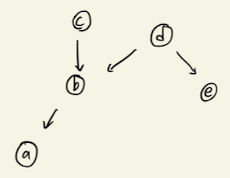
Let's assume we have a direct graph as below.

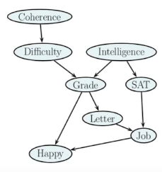
The joint probability of all the variables in the graph is given by,

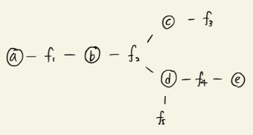
Now through the process of message passing, we have moralized the graph as follows.

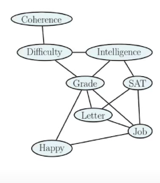
And the joint probability of the undirected graphical model is given by,

Now we pick an ordering in which we desire to remove random variables.

Factor Graph

• Factor graph is a graphical model representation that unifies directed and undirected models
• Undirected bipartite graph with two kinds of nodes
  - Round nodes represent variables
  • Square nodes represent factors
• There is an edge from each variable to every factor that mentions it.

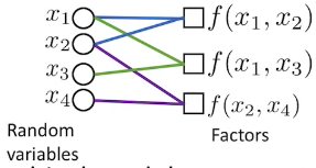
• Variables:
  $X=\{X_1,...,X_i,...,X_n\}$
• Factors:
  $\psi_a, \psi_b, \psi_c, ...$, where $a,... \sub \{1,...,n\}$
• Joint Distribution (Gibbs Distribution):
  $p(x)=\frac 1 Z \prod_\alpha \psi_\alpha(x_\alpha)$
  

Inference Example

Consider a directed graph below.

The joint probability of the directed graph above is represented as follows.

We can moralize the directed graph as the following.

The undirected graph above can be factorized as the following.

• How would we calculate $p(a,b)?$
  $p(a,b)=f_1(a,b)\sum_{c,d}f_2(b,c,d)f_3(c)f_5(d)\sum_ef_4(d,e)$
• Note that $f_1(a,b)=P(a|b)$ and $f_4(d,e)=P(e|d)$
• Note that $\sum_e f_4(d,e) = m_e(d)$
• Note that $f_5(d)=m_d(d)$

Message passing in Belief Propagation

• $\psi$, an unnormalized function of the dependence relation.
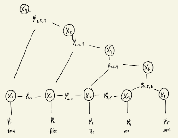
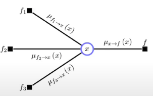
• Conceptually, we can view $\psi$ as a message passed on from other nodes onto a node. Image below gives an intuition of message passing.

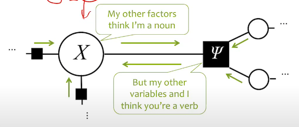
• A "belief" in $X_1$ is basically a product of all the incoming factor $\psi_1 * \psi_2 * \psi_3$.

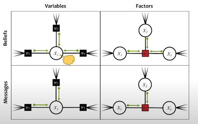
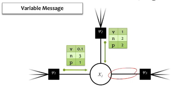
Variable Belief

Variable Message

The equation above means that the outbound message from a node is equal to the product of all the inbound messages.

Factor Belief

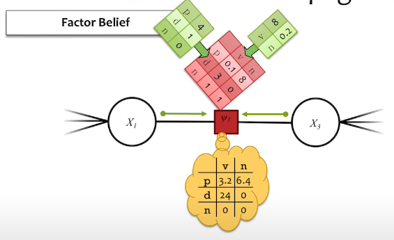
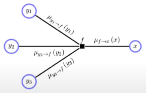
Factor Message

Where $\alpha$ is the index of message sending node, and $i$ is the index of node that receives message.
The equation above means that the message of a factor from node $\alpha$ to node $i$ is (1) product of all the inbound messages, (2) product of factor value to (1), (3) integrate(sum) out all the un-necessary variables.

On the example below, the process is described by the following.

• (1) factor $\psi_1$ receives message from the node $X_3$.
  $\mu_{x_3\rightarrow \psi_1}$
• (2) Factor $\psi_1$ applies the CPD onto the message.
  $\psi_1 * \mu_{x_3\rightarrow \psi_1}$
• (3) Integrate out all the unnecessary variables with regards to $X_1$
  $\sum_{x_3}\psi_1 * \mu_{x_3\rightarrow \psi_1}$
  The equation above shows the message passing from node $X_3\ to\ X_1$.

Summary of the Messages

Variable to Factor message

Factor to Variable message

Where the first part of the equation (max term) is a process of integrating out all the unnecessary variables.

Sum-Product Belief Propagation

Input: a factor graph with no cycles
Output: exact marginals for each variable and factor.

Algorithm:
1. Initialize the messages to the uniform distribution

1. Choose a root node
2. Send messages from the leaves to the root.
   Send messages from the root to the leaves.
   $\mu_{i\rightarrow \alpha}(x_i)=\prod_{\alpha \in N(i)\backslash\alpha} \mu_{\alpha \rightarrow i}(x_i)$
   $\mu_{\alpha \rightarrow i}(x_i)=\sum_{x_{\alpha}:x_{\alpha}[i]=x_i}\psi_\alpha(x_\alpha)\prod_{j\in N(\alpha)\backslash i}\mu_{j \rightarrow \alpha}(x_\alpha[i])$
3. Compute the belief (unnormalized marginals)
   $b_i(x_i)=\prod_{\alpha \in N(i)}\mu_{\alpha \rightarrow i}(x_i)$
   $b_\alpha(x_\alpha)=\psi_\alpha(x_\alpha) \prod_{i \in N(\alpha)} \mu_{i \rightarrow \alpha}(x_\alpha[i])$
4. Normalize beliefs and return the exact marginals.
   $p_i(x_i) \propto b_i(x_i)\\ p_\alpha(x_\alpha) \propto b_\alpha(x_\alpha)$

Loops make issues in Message Passing

Recall that message Passing requires leaf nodes in order for the (forward, backward) propagation to end.

Suppose we have a graph given by

If we eliminate variables, the graph becomes

Which is still a connected graph.

Clique Graph

Def
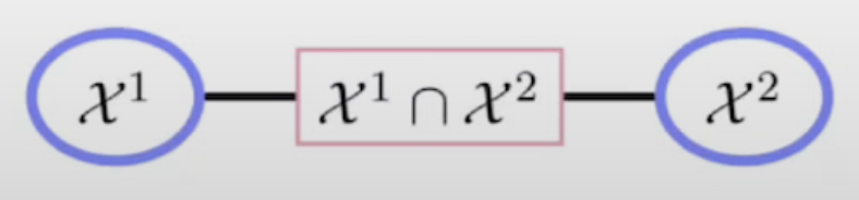
A clique graph consists of a set of potentials, $\phi_1(\chi_1),...,\phi_n(\chi_n)$ each defined on a set of variables $\chi_1$. For neighboring cliques on the graph, defined on sets of variables $\chi_1, \chi_j$, the intersection $\chi_s=\chi_i\cap\chi_j$ is called the separator and has a corresponding potential $\phi_s(\chi_s)$.

A clique graph represents the function,

Example

$\phi(\chi^1)\phi(\chi^2)/\phi(\chi^1\cap\chi^2)$

Example: Probability density
Let's assume we have a graph as following.

Proof Summary

By Definition.
Multiplying both equations,

Junction Tree

• Form a new representation of the graph in which variables are clustered together, resulting in a singly-connected graph in the cluster variables.

• Distribution can be written as product of marginal distributions, divided by a product of the intersection of the marginal distributions.

• Not a remedy to the intractability.

• We can obtain Junction Tree through variable elimination process.

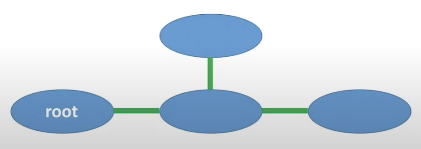
• The message passing protocol
  Cluster B is allowed to send a message to a neighbar C only after it has received messages from all neighbors except C.

Pseudo Code

def Collect(C):
	for B in children(C):
    	Collect (B)
        send message to C
        
def Distribute(C):
	for B in children(C):
    	send message to B
        Distribution(C)

Message from Clique to another

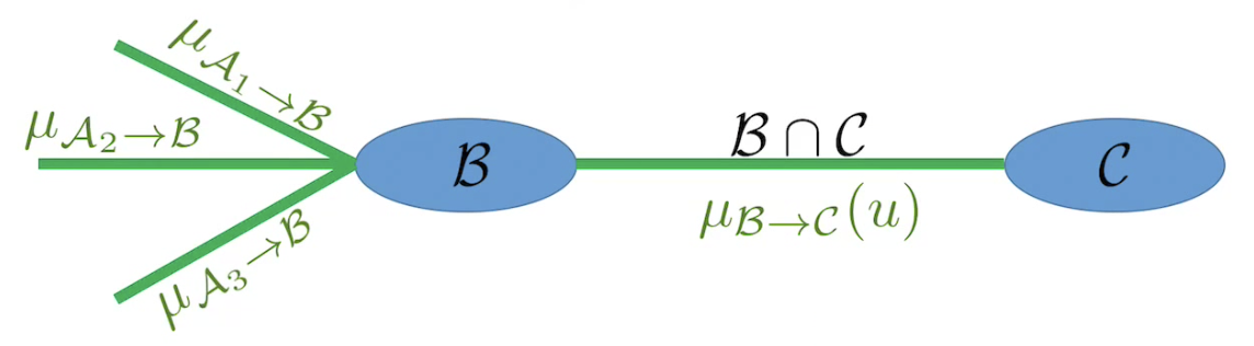
The graph above is Message Passing protocol from Cluster $B$ to Cluster $C$.
Cluster $B$, $C$ have their own sets of random variables in their Clusters (or Cliques).
$B\cap C$ is a set of random variables that are shared between the two clusters.

In short, the procedure is the following.
1. B Collects all the incoming messages
2. B Applies its own factor ($\psi_B$ in the equation above)
3. Integrade all the random variables that C doesn't understand (i.e. C does not include)

Formal Junction Tree Algorithm

1. Moralization: Marry the parents (only for directed distributions).
2. Triangulation: Ensure that every loop of length 4 or more has a chord. In other words, every loop must have a minimal clique of size 3.
3. Junction Tree: Form a junction tree from cliques of the triangulated graph, removing any unnecessary links in a loop on the cluster graph. Algorithmically, this can be achieved by finding a tree with maximal spanning weight with weight given by the number of variables in the separator between cliques. Alternatively, given a clique elimination order, one may connect each clique to the single neighboring clique.
4. Potential Assignment: Assign potentials to junction tree cliques and set the separator potentials to unity.
5. Message Propagation

Some Facts about Belief Propagation

• BP is exact on trees. (No approximation)
• If BP converges it has reached a local minimum of an objective function (No proof of convergeance, though)
• If it converges, convergence is fast near the fixed point.

Zoo of Network

UGM and DGM

• Use to represent family of probability distributions
• Clear definition of arrows and circles

Factor Graph

• A way to represent factorization for both UGM and DGM
• Bipartite Graph
• More like a data structure
• Not to read the independencies (i.e. no functionality of I-Map)

Clique graph or Junction Tree

• A data structure used for exact inference and message passing
• Nodes are cluster of variables
• Not to read the independencies (i.e. no functionality of I-Map)