Exact Inference

• Inference
  Used to answer queries about $P_M,\ e.g.,\ P_M(X|Y)$

• Learning
  Used to estimate a plausible model $M$ from data $D$

Query

1. Likelihood

• Evidence $e$ is an assignment of values to a set $E$ variables in the domain.
• $E=\{X_{k+1},...,X_n\}$
• Simplest query:
  $P(e)=\sum_{x_1}...\sum_{x_2}P(x_1,...,x_k,e)$
• this is often referred to as computing the likelihood of $e$
• Notice that $E$ and $X_1,...,X_k$ are disjoint set.

2. Conditional Probability

$P(X|e)$ is the a posteriori belief in $X$, given evidence $e$.

• Marginalization: the process of summing out the "unobserved" or "don't care" variables z is called.
  $P(Y|e)=\sum_z P(Y,Z=z|e)$

3. Most Probable Assignment

• most probable joint assignment (MPA) for some variables of interest.
• What is the most probable assignment of
  $max_{x_1,...,x_4}P(x_1,...,x_4|e)?$
  where $e$ is the evidence, and $x_1,...,x_4$ are random variables of interest?
  $MPA(Y|e)=arg\ max_{y\in Y}\ P(y|e)=arg\ max_{y\in Y} \sum_z P(y,z|e)$
• maximum a posteriori configuration of $Y$.
• Used in classification / explanation tasks.

example)

Now we want,

How can we compute the Posterior Distribution?

Applications of A Posteriori Belief

• Prediction: what is the probability of an outcome given the starting condition?
  $A => B => C$
  $P(C|A)?$
• Diagnosis: what is the probability of disease/fault given symptoms?
  $A => B => C$
  $P(A|C)?$

Landscape of inference algorithms

Exact inference algorithms (Classical)

• Elimination algorithms
• Message-passing algorithms (sum-product, belief propagation)
• Junction tree algorithms

Approxmiate inference techniques (Modern)

• Stochastic simulation / sampling methods
• Markov chain Monte Carlo methods
• Variational algorithms

Variable Elimination

• Query: $P(e)$
  $P(e)=\sum_d \sum_c \sum_b \sum_a P(a,b,c,d,e)\\ = \sum_d \sum_c \sum_b \sum_a P(a)P(b|a)P(c|b)P(d|c)P(e|d)$
• Eliminate nodes one by one all the way to the end,
  $P(e)=\sum_d P(e|d)p(d)$
  The computational complexity of the chain elimination is $O(n*k^2)$ where $n$ is number of elimination steps, and $k$ is the dimension of the Vector.

Example) Markov Chain
Let transition matrix M be a 3x3 matrix in a markov chain, where there are three states.

• Let $X$, nodes in a markov chain be the state that
• What is the probability distribution of a random walk the the transition matrix, M?
  $p(x_5=i|x_1=1)=\sum_{x_4,x_3,x_2} p(x_5|x_4)p(x_4|x_3)p(x_3|x_2)p(x_2|x_1=1)\\ = [M^4v]_i$
• What is the probability distribution of a random walk when $t \rightarrow \infty$?
  If we denote the stationary distribution as $\pi$,
  $\pi M = \pi$
  The problem formation above looks similar to the eigenvalue decomposition form, $Mv=\lambda v$, with $\lambda=1$.
  $(\pi M)^T \rightarrow M^T\pi^T=1*\pi^T$
  In other words, the transposed transition matrix $M^T$ has eigenvectors as $\pi^T$ with eigenvalue of $1$.

We can find the stationary distribution of a given transition matrix through eigenvalue decomposition of the transition matrix. Stationary distribution is the eigenvector with $\lambda=1$.

Message Passing

• Doesn't work in a cyclical graph
  Message backpropagation can be stuck in a cycle.
• Variable Elimination through Message Passing allows us to marginalize out unnecessary variables, with better Complexity.

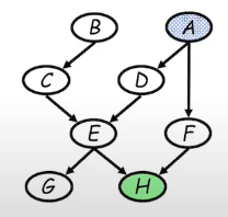
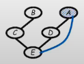
Example: Variable Elimination

• Given the graph above, what is the posterior probability, $P(A|h)?$

• Initial factors:

  $P(a,b,c,d,e,f,g)=P(a)P(b)P(b|c)P(d|a)P(e|c,d)P(f|a)P(g|e)P(h|e,f)$

  Joint probability factorizes in such manner because the graph is a directed model.

• Choose elimination order: $H,G,F,E,D,C,B$

• Step1:
  - Conditioning (fix the evidence node $h$ on its observed value $\tilde h$

  $m_h(e,f)=p(h=\tilde h|e,f)\\ m_h(e,f)=\sum_h p(h|e,f)\sigma(h=\tilde h)$

  where $\sigma(h=\tilde h)$ is a dirac-delta function.
  So far we have removed $P(h=\tilde h|e,f)$, and introduced a new term $m_h(e,f)$. Now $e$ and $f$ become dependent.
  Through introducing a term for Message Passing, we are essentially converting a Directed Graphical Model to an Undirected Graphical Model.

  Delta function is a function with 1 on the value that the observation h holds and 0, otherwise.

Now,

• Step2:
  -Eliminate G
  Since there is no term that depends on $G$, we can eliminate $G$ without having to introduce any new message factor.
  $m_g(e)=\sum_g P(g|e) = 1$

• Step3:
  -Eliminate F
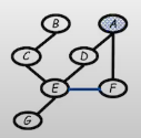
  If we eliminate $F$, we need to connect $(E, A)$ together, since a new factor will be introduced to make them dependent.

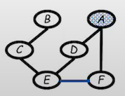
• Step4:
  -Eliminate E
  $m_e(a,c,d)=\sum_e p(e|c,d)m_f(a,e)$

• Step5:
  -Eliminate D

• Step5:
  -Eliminate C

• Step6:
  -Eliminate B

  $m_b(a)=\sum_b p(b)m_c(a,c)$

• Final Step:
  -Wrap-up
  We have created message passing from $A$ to $H$, using graph elimination. Since the initial state we were eliminating from was the joint distribution of the variables in the graph, we can finally calculate the conditional distribution, $P(a|\tilde h)$.

• Complexity Analysis
  If we were to integrate every single variables, the complexity would be $O(K^6)$, since we are marginalizing out 6 Variables. However, through Message Passing, at each step the complexity would be $O(K^2)$, resulting in total of $6*O(K^2)$

Overview of Graph elimination

• Begin with the undirected GM or moralized Bayesian Network (meaning changing the Directed Graph to an Undirected Graph.

• Graph $G(V, E)$ and elimination ordering $I$

• Eliminate next node in the ordering $I$
  - Removing the node from the graph

  • Connecting the remaining neighbors of the nodes

• The reconstituted graph $G'(V,E')$
  - Retain the edges that were created during the elimination procedure

  • The graph-theoretic property: the factors resulted during variable elimination are captured by recording the elimination clique. (Notice that Intermediate terms of form $m_x(Y, Z)$ correspond to the cliques resulted from elimination.