Recap

Exponential Family

• $A(\theta)$ is called log partition function.
• $T(x)$ is called sufficient statistics.
• $A(\theta)$ is convex.
• $A(\theta)$'s first derivative with respect to $\theta$ is Expectation of $T(x)$, and second derivative with respect to $\theta$ is the Variance of $T(x)$.
• Since $A(\theta)$ is (1) a function of the natural parameter, $\theta$, (2) convex function, we can solve the following equation, and obtain an expression for the natural parameter, $\theta$ using the moment parameter, $\mu$.
  $\frac{d}{d\theta} A(\theta)=\mu\\$
  Solving for $\theta$, we can obtain,
  $\theta=\psi(\mu)$

In short, for a random variable $X$ that is from natural exponential family distribution, the moment generating function is given by the following:

	-Note that natural exponential family distribution has sufficient statistics, T(x)=x

Recall that the definition of Moment Generating Function is given as follows

Applying the moment generating function to T(x),

Furthermore,

---

• MLE (Maximum Likelihood Estimation) for exponential family is the same as moment matching.
  (a) Log likelihood of a generic exponential family: $const + \theta^T(\sum T(x_i)) - nA(\theta)$
  (b) Taking the gradien w.r.t. $\theta$: $\sum T(x_i) - n \Delta_\theta A(\theta)$
  (c) Setting equal to zero and solving for $\Delta_\theta A(\theta)$: $\Delta_\theta A(\theta) = \frac 1 n \sum T(x_i) \rightarrow \mu = \frac 1 n \sum T(x_i)$

Bayesian POV

After writing down the likelihood of the dta given the natural parameter, we want to pick a prior over the natural parameter, and work out the posterior over the natural parameter.

Generalized linear models (GLIM)

Components

• Linear predictor: Linear function of regressors,
  $\lambda_i=\alpha + \beta_1 X_{i1}+...+\beta_kX_{ik}$
• Link function: Transforms the expectation of the response variable, $\mu_i=E(Y_i)$ to the linear predictor. In other words, the link function linearizes the expectation of the response variable:
  $g(\mu_i)=\lambda_i=\alpha + \beta_1 X_{i1}+...+\beta_kX_{ik}$
• Because the link function is invertible, we can write
  $\mu_i=g^{-1}(\lambda_i)=g^{-1}(\alpha + \beta_1 X_{i1}+...+\beta_kX_{ik})$

Assumptions

where $Y$ are the responses, $x$ are the fixed inputs, $\theta$ are parameters we need to learn, and $f$ and $\psi$ give us added flexibility if we want it.

Graphical Representation of GLM Models

We can describe the process as the following graph.

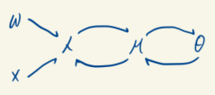
• $W$ are the parameters.
• $\lambda = W^TX.$
• $\mu$ is called standard parameters, and signifies the mean of $Y|X.$
• $\theta$ is called natural parameters, that governs the shape of the density $Y|X$. It can be the case that $\mu=\theta\ (e.g., normal),$ but this doesn't need to be true (Poisson distribution, for example).
• We are aiming to model a transformation of the mean, $\mu$ by finding $g(\mu)$ that satisfies $\theta=g(\mu)=\lambda(X)=W^TX.$

MLE for Undirected Graphical Models###

1. Data

2. Model
In a typical setup for Undirected Graphical Models, it is bett

3. Objective

4. Learning

5. Inference

• Marginal Inference; Inference over the variables of interest.
  $p(x_c)=\sum_{x':x'^c=x_c} p(x'|\theta)$
• Partition Function; Normalizing function for the Gibbs distribution obtained by factorization.
  $Z(\theta)=\sum_x \prod_{C \in c}\psi_C(x_C)$
• MAP Inference; Compute variable assignment with highest probability.