UGM Inference

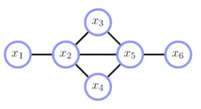
• Graphical model structure is given
• Every variable appears in the training examples (no unobserved)

Questions

1. What does the likelihood objective accomplish?
2. Is likelihood the right objective function?
3. How do we optimize the objective function?
4. What guarantees does the optimizer provide?
5. What is the mapping from data to model? In what ways can we incorporate our domain knowledge? How does this impact learning?

Settings

1. $\psi_C(x_C)=\theta_{C,x_C}$

• Random Variables are discrete.
• Parameters are the connection between the nodes.
• MLE by inspection (Decomposable Models).
• Iterative Proportional Fitting (IPF).

ex) If there is only 1 node in a clique, the parameters will be a vector. If there are 2 nodes, the parameters will be a matrix. If there are 3 nodes, the parameters will be a Tensor of 3 dimension, etc.

2. $\psi_C(x_C)=exp(\theta*f(x_C))$

• Random Variables are continuous.
• Generalized Iterative Scaling.
• Gradient-based Methods.
• $\theta$ are the parameters, and $f(x_c)$ is some feature function.

Let $D=\{\vec{x_1},..., \vec{x_n}\}$ the observed data, $\vec{x}^{i.i.d.} \sim p(\vec{x};\theta)$
Now, MLE is given by:

where each clique is denoted as $c$, $Z(\theta)$ is a normalizing constant.

Then,

Taking Derivative with respect to $\theta_c$ and setting the value to zero, we obtain

Since the first term is empirical mean, and the second term is the true mean, we thus have that the true mean equals to the empirical mean.

Decomposable Graphs

By Junction Tree Algorithm,

Intuition
Let's assume we have a graph as follows.

Now if we apply the Junction Tree Algorithm, we get the joint probability expressed as the following graph.

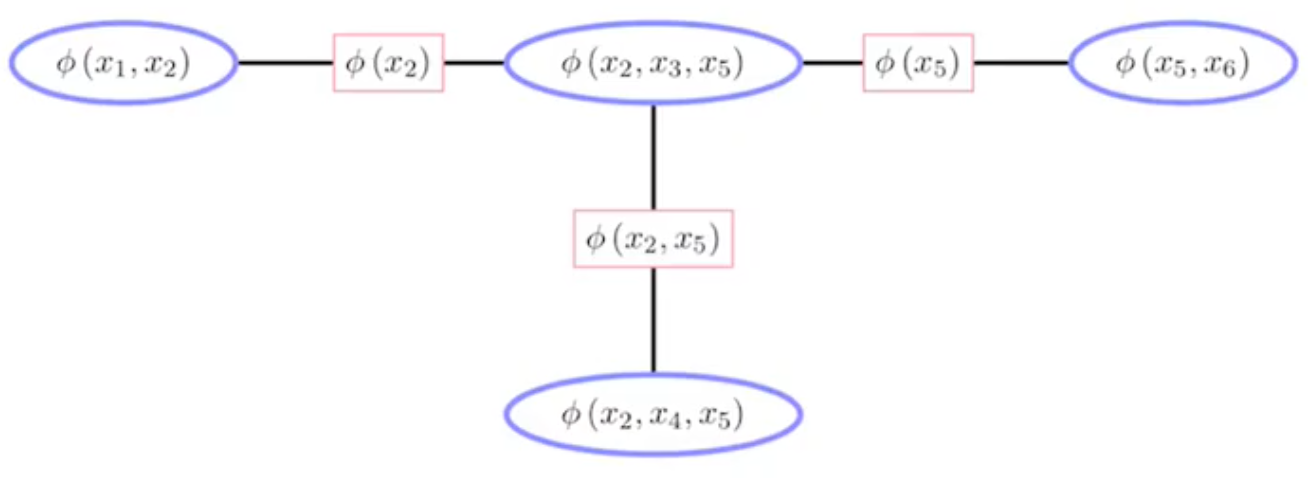
Rewriting the RHS of the equation above, we obtain

Which is, expressed in an un-normalized form,

Now the Loss becomes

IPF update

• Iterates a set of fixed-point equations
• Fixed-point update means setting the equation at the desired point, assign the updated values, and iterate over.

Where $\epsilon(y_c)$ is empirical marginal distribution of $y_c$,
$p^{(t)}(y_c)$ comes from inference of the graph with the currently updated parameters. i.e., $p^{(t)}(y_c)=\sum_{y':y'_c=y'_c} p(y';\theta^{(t)})$

Feature-based Clique Potentials

• For large cliques these general potentials are exponentially costly for inference and have exponential numbers of parameters that we must learn from limited data.
• Could make cliques smaller, but this changes the dependencies.
• Keep the same graphical model, but use a less general parameterization of the clique potentials.
• Feature based models.

Features

• Consider a clique $x_c$ of random variables in a UGM; three consecutive characters $c_1c_2c_3$ in a string of English text.

• How would we build a model of p(c_1,c_2,c_3)?
  If we use a single clique function over $c_1c_2c_3$, the full joint clique potential would be huge;(26^3-1) parameters. However, we often know that some particular joint settings of the variables in a clique are quite likely or quite unlikely; "ing", "ion",...

• A "feature" is a function which is vacuous over all joint settings except a few particular ones on which it is high or low.
  For example, we might have $f_{ing}(c_1,c_2,c_3)$ which is 1 if the string is 'ing' and 0 otherwise, and similar features for 'ion', etc..

• Typically we can let features represent any of our prior knowledge over the cluster, and we can utilize the features to represent the potential function coming from each clusters.

Features as Micropotentials

• By exponentiating them, each feature function can be made into a "micropotential". We can multiply these micropotentials together to get a clique potential.
• Example: a clique potential $\psi(c_1,c_2,c_3)$ could be expressed as:
  $\psi_c(c_1,c_2,c_3)=e^{\theta_{ing}f_{ing}}*...$

• This is still a potential over $26^3$ possible settings, but only uses K parameters if there are K features.
  Note that by having one indicator function per combination of $x_c$, we recover the standard tabular potential.

• Each feature has a weight $\theta_k$ which represents the numberical strength of the feature and wheter it increases or decreases the probability of the clique.

• The marginal over the clique is a generalized exponential family distribution, actually, a $GLM$

• In fact, by using such defined setup, we can see that

  $p(c_1,c_2,c_3)=\frac 1 {Z(\theta)} \prod_c exp(\theta_c^Tf(x_c))\\ = exp(\sum_c \theta_c^T f_c(X_c) - logZ(\theta))$

  which is, as a result, an exponential family.

• Therefore, the joint probability model now becomes an exponential family, if we define each Clique Potential to be defined that way.

• In general, the features may be overlapping, unconstrained indicators or any function of any subset of the clique variables:

Expressing the clique potentials with feature functions, we can write

• Can I use IPF?
  Not exactly, but we can make modification to that.
  

Generalized Iterative Scaling (GIS)

Key Idea:
- Define a function which lower-bounds the log-likelihood
- Observe that the bound is tight at current parameters
- Increase lower-bound by fixed-point iteration in order to increase log-likelihood

** This Idea is akin to a standard derivation of the Expectation-Maximization Algorithm.

IPF vs GIS

• IPF is a general algorithm for finding MLE of UGMs.
  $\phi^{(t+1)}_c(y_c) \leftarrow \phi^{(t)}_c(y_c)\frac{\epsilon(y_c)}{p^{(t)}(y_c)}$
• GIS is iterative scaling on general UGM with feature-based potentials.
• IPF is a special case of GIS which the clique potential is built. on featurers defined as an indicator function of clique configurations.

The two methods are essentially using the same logic;
Set next update to be current update + $\frac {empirical} {marginal}$