UGM (Undirected Graphical Model)

Random Field

Defn
A random field is a random function over an arbitrary domain. i.e. it is a function $f(x)$ that takes on a random value at each point $x\in R^n$. By modern definitions, a random field is a gneralization of a stochastic process where the underlying parameter can take multidimensional vectors or points on some manifold.

Markov Random Field (Markov Network)

Defn
A set of random variables having a Markov property described by an undirected graph. i.e. a random field that satisfies Markov Properties.

• Equivalent of Undirected Graphical Model.
• Directed Graphical Models are called Bayesian Network.

Markov Properties

• Global Property
  Consider disjoint subsets $A,B,$ and $C$ of the Markov Network. $A$ and $C$ are conditionally independent given $B$ iff all paths connecting $A$ and $C$ pass through $B$.
• Local Property
  A node is conditionally independent from the rest of the network given its neighbors.
• Pairwise Property (Also called Markov Blanket Property)
  Any two nodes in the Markov network are conditionally independent given the rest of the network if they are not neighbors.

Gibbs Random Field

Defn
When the joint probability density of the random variables in Markov Random Field is strictly positive, it is also referred to as a Gibbs random field.

Intuition of Why
Hammersley-Clifford theorem states that the strictly positive probability density can be represented by a Gibbs measure for an appropriate energy function.

Markov Network

For a set of variables $X=\{x_1,...,x_n\}$ a Markov network is defined as a product of potentials on subsets of the variables $X_c \subset X$

Where,

• $\phi_c$ is called potential $\geq 0$ (this does not have to be probability)
• $X_c$ is Maximal clique
• $Z$ is a normalizing factor to scale the product value to be within range $[0,1]$

Difference between Markov Network and Bayesian Network

• Markov networks allow symmetrical dependencies between variables (undirected graphical model).
• Markov networks allow cycles, and so cyclical dependencies can be represented.

Conditional Independence:

Global Markov Property: $X_A\perp X_B | X_C$ iff $C$ separates $A$ from $B$ (there is no path connecting them). This is also referenced as Gibbs Distribution.

Markov Blanket(local property): The set of nodes that renders a node $t$ conditionally independent of all the other nodes in the graph.

where $V$: All nodes in the graph.
$mb(t)$: Markov Blanket.

Clique

Defn
A clique is a subset of vertices of an undirected graph such that every two distinct vertices in the clque are adjacent. i.e, there exists edge for every two vertices in undirected graph.

Example 1)

Example 2)

Example 3)

Clique Potential
Cannot interpret $\phi$ as marginals or conditionals.
Can only be interpreted as general "compatibility" or "relationship" over their variables, but not as probability distributions.

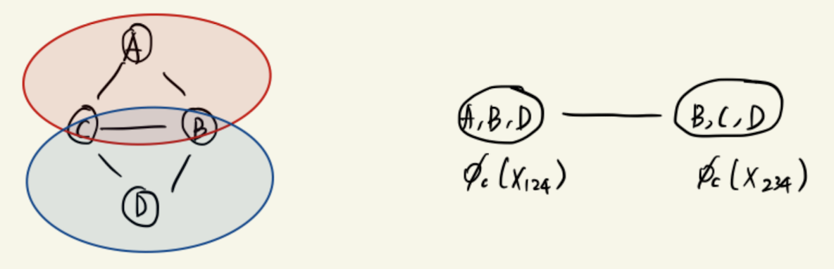
Maximal Clique

Defn
A maximal clique is a clique that cannot be extended by including one more adjacent vertex, meaning it is not a subset of larger clique.

UGM representation

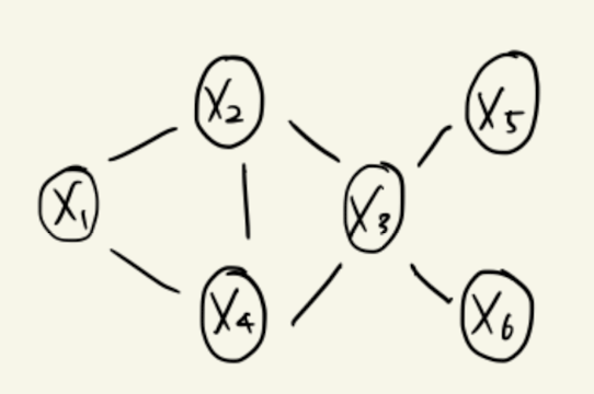
Example)

1. Maximal Clique Representation

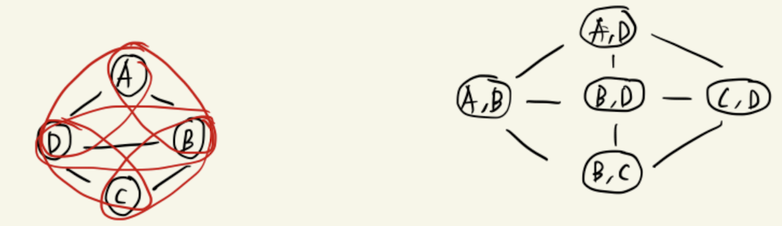
2. Sub-Clique Representation: Pairwise MRFs

• Two graphs, $P'$ and $P''$ have equivalent I-maps, i.e. $I(P') == I(P'')$ since both factorization is coming from the graph itself.

Hammersley-Clifford Theorem

• If arbitrary potentials are utilized in the following product formula for probabilities,

  $P(x_1,...,x_n)=\frac 1 Z \prod_{c\in C}\phi_c(x_c)\\ Z=\sum_{x_1,...,x_n}\prod_{c\in C}\phi_c(x_c)$

  then the family of probability distributions obtained is exactly that set which respects the qualitative specification (conditional independence relations) described earlier.

• Thm: Let P be a positive distribution over V, and $H$ a Markov network graph over V. If $H$ is an I-map for P, then P is a Gibbs distribution over $H$.

• The theorem states that the process is a Markov random field iff the corresponding joint distribution of the graph is a Gibbs distribution.

Proof
Let $\{X_t:t\in T\}$ be a finite collection of random variables with $X_t$ taking values in a finite set $S_t$. Let the index set $T$ be $\{1,...,n\}$ and $S_t=\{0,...,m_t\}$. The joint distribution of the variable is

with $0\leq x_t \leq m_t$. The vector $X=(X_1,...,X_n)$ takes values in $X=\prod_{t\in T} S_t$, the set of all n_tuples $x=(x_1,...,x_n)$ with $x_t\in S_t$ for each $t$.
Suppose $T$ is the set of nodes of a graph. Let $N_t$ denote the set of nodes (the neighbors of $t$) for which $(t,s)$ is an edge of the graph.

Definition
The process is said to be a Markov random field if
(i) $Q\{x\}\gt 0$ for every $x$ in $X$
(ii) for each $t$ and $x$,

Which simply means that the conditional probability of a node is independent of all other nodes in the graph given its neighbors.

A subset $A$ of $T$ is said to be complete if each pair of vertices in $A$ defines an edge of the graph. $\Gamma$ doesnotes the collection of all complete subsets. Clique is another terminology for complete graph.

Definition
The probability distribution $Q$ is called a Gibbs distribution for the graph if it can be written in the form

where each $V_A$ is a positive function that depends on $x$ only through the coordinates $\{x_t:t\in A\}$.

The Hammersley-Clifford Theorem asserts that the process $\{X_t:t\in T\}$ is a Markov random field iff the corresponding $Q$ is a Gibbs distribution.

Factor Graphs

• A factor graph is a graphical model representation that unifies directed and undirected models.
• Bipartite Graph is composed of Circle Nodes and Square Nodes in the Graph.
• Round Nodes represent Random Variables of the Graph
• Square Nodes represent factors of the Graph. i.e. relationship between the nodes; edges in the graph.

Example)
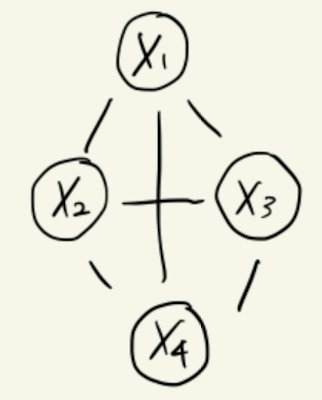
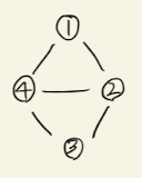
Original UDG is Given by the following, where vertices 1~4 are Random Variables, edges are dependence relationship.

• 

• 

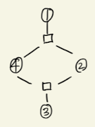
The graph above represents factorization by

where $Z$ is a normalization constant.

• 

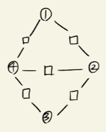
The graph above represents factorization of the original UDG by

where $Z$ is a normalization constant.

Example for DGM

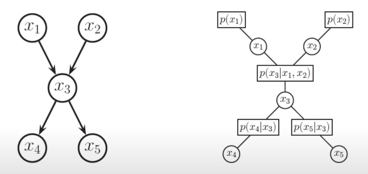
The DGM above can be interpreted as follows.

Directed Graphical Model is a subset of UDG. And therefore, the factor graph we have established above can be applied to the directed graphical model. Furthermore, unlike UDG, DG's dependence relationship can be identified by probability, since there is a unique way how a DG is interpreted.
If the graph above were to be a UDG the joint probability would be given by the following.

Practical Examples

Exponential Form

• Gibbs Distribution
  $p(x_1,...,x_n)=\frac 1 Z \prod_{c=1}^C \phi_c(X_c)$
  And $\phi_c(X_c)$ is called Potentials.

We are free to define $\phi$ function differently, as long as the function meets the requirement of non-negative function. Therefore, we can represent the distribution using exponential term.

Free energy of the system (log of prob):

Powerful parametrization (log-linear model):

where, $f_c(X_c)$ term is feature function, and $\theta_c$ is probability of theta.

Boltzmann Machines
A fully connected graph with pairwise potentials on binary-valued nodes is called a Boltzmann machine.
We want to find what is the most stable system.

Where one can think of the first term $\sum_{ij}\theta_{ij}x_ix_j$ as binary term, $\sum_i\alpha_ix_i$ as unary term, and $\theta_{ij}$ and $\alpha_i$ are parameters associated.

Therefore, overall energy function has a quadratic form.

Since the objective is to find the most stable system, finding the minimum energy state is the objective of the Boltzmann machine. Since the energy function has. aquadratic form, we can simply find the minima for $H(x;\theta,\mu)$, if $\theta,\alpha$ are known.

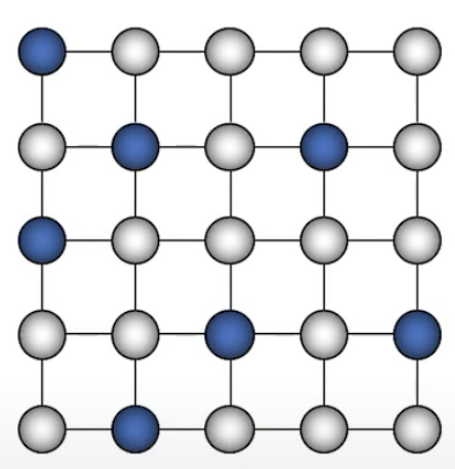
Ising Models

• Nodes are arranged in a regular topology and connected only to their geometric neighbors.

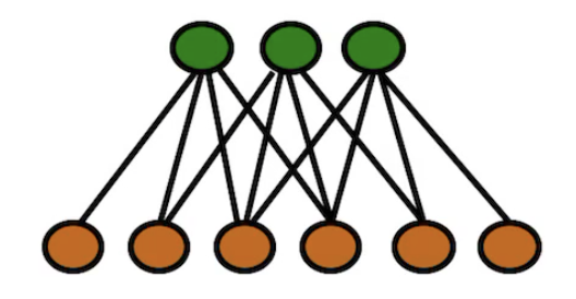
Restricted Boltzmann Machines (RBM)

• Observed are data

• Unobserved has "a notion" of summary of data

  $p(x,h;\theta)=exp\bigg(\sum_i\theta_i \phi_i(x) + \sum_j \theta_j \phi_j(h_j) + \sum_{i,j} \theta_{i,j}(x_i,h_j) - A(\theta) \bigg)$

• Factors are marginally dependent.

• Factors are conditionally independent given observations on the visible nodes.

  $p(h_1,...,h_M|x)=\prod_m p(h_m|x)$

• Iterative Gibbs sampling to generate pairs of (x,h).

Conditional Random Fields (CRF)

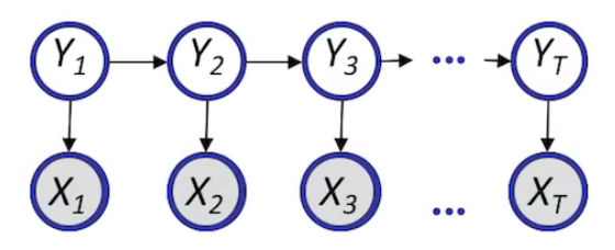
• An example of log linear model.