---

개요

머신러닝의 기본 정의 및 종류

---

📌 2회차 요약

• 회귀 분석 > 선형 회귀

---

📌 선형 회귀

---

📌 용어 정리

• 공통

  • Y 는 종속 변수 또는 결과 변수
  • X 는 독립 변수 , 원인 변수 또는 설명 변수

• 통계학에서 사용하는 선형회귀 식

  $Y = \beta_0 + \beta_1X + \varepsilon$
  • $\beta_0$ : 편향(Bias)
  • $\beta_1$ : 회귀 계수
  • $\varepsilon$ : 오차(에러), 모델이 설명하지 못하는 Y의 변동성

• 머신러닝 / 딥러닝에서 사용하는 선형회귀 식

  $Y = wX + b$
  • $w$: 가중치
  • b: 편향(Bias)

두 수식이 전달하려고 하는 의미는
회귀 계수 혹은 가중치 값을 알면 X 가 주어졌을 때 Y 를 알 수 있다는 것.

---

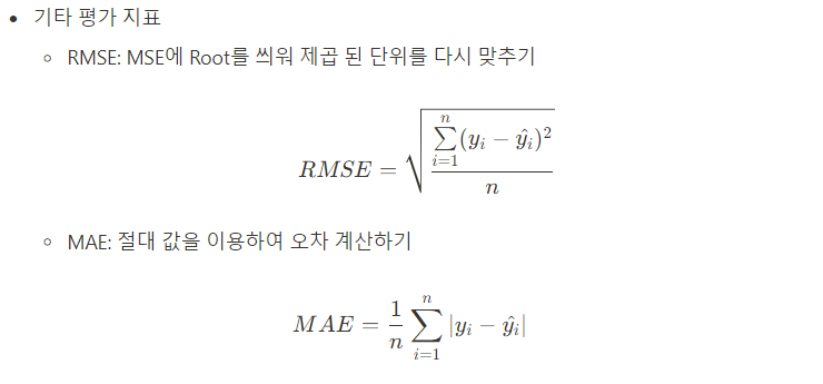
📌 회귀 분석 평가 지표

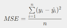
MSE

1. 에러 정의 = 실제 데이터 - 예측 데이터
2. 에러를 제곱하여 모두 양수로 만들고 다 합치기
3. 데이터만큼 나누기

에러 정의 과정 수식화
1. 에러 정의 : $\varepsilon = y_i - \hat{y_i}$
2. 제곱하여 합치기 : $\sum\limits_{i=1}^n (y_i - \hat{y_i})^2$
3. 데이터만큼 나누기 : $\frac{\sum\limits_{i=1}^n (y_i - \hat{y_i})^2}{n}$

위 에러를 Mean Squared Error (MSE) 라고 정의

+)

---

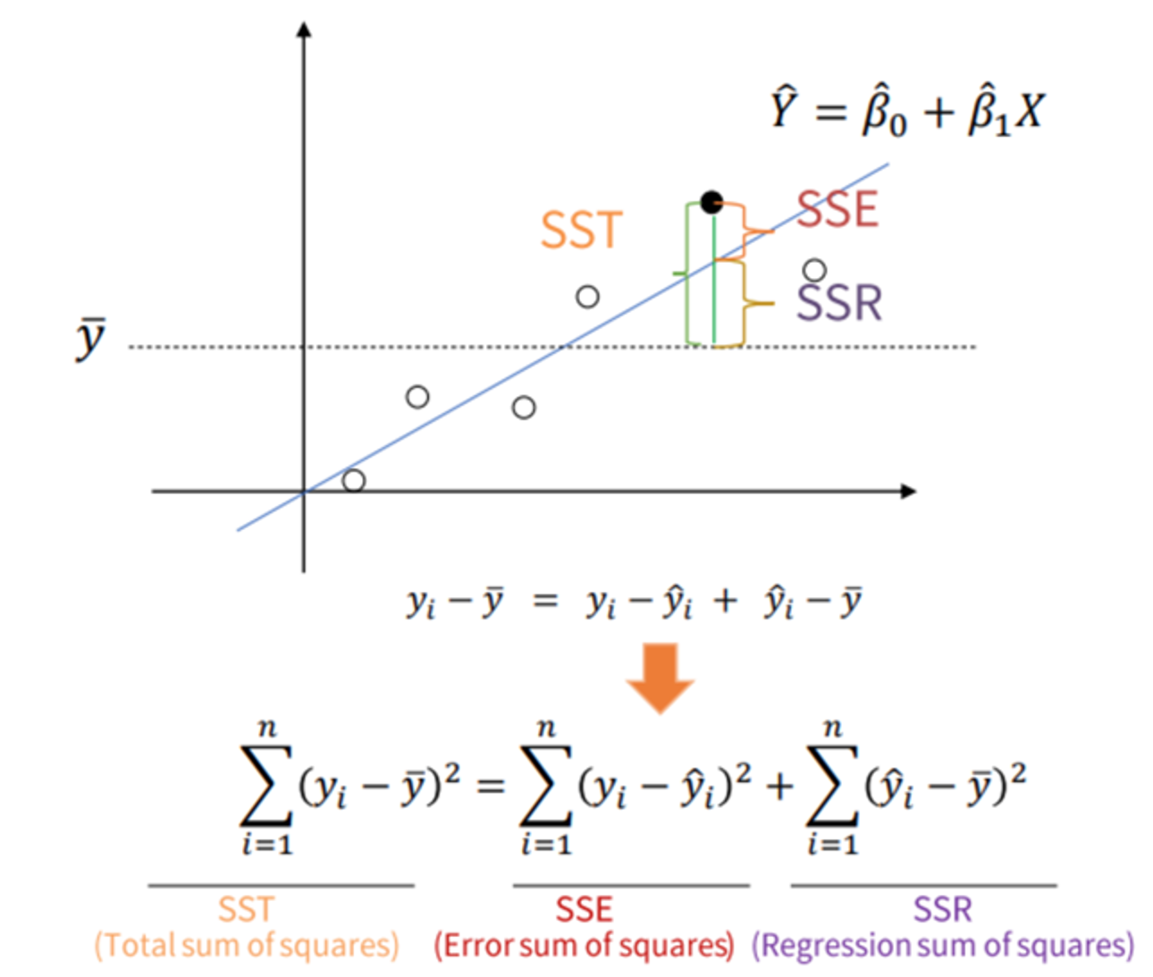
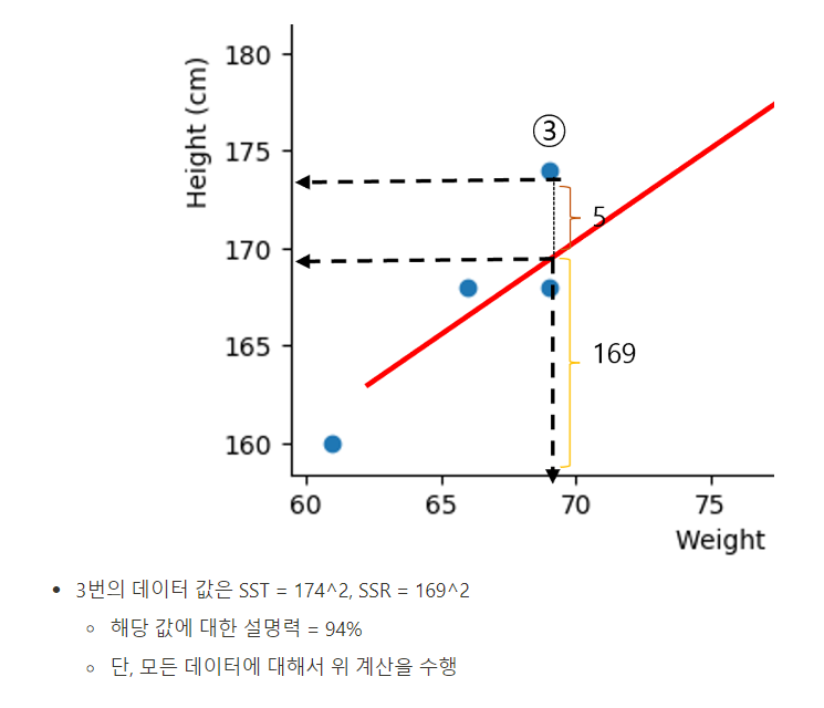
선형회귀만의 평가 지표 - R Square

• 숫자를 예측하는 회귀분석에서, 선형 회귀에서만 평가되는 지표
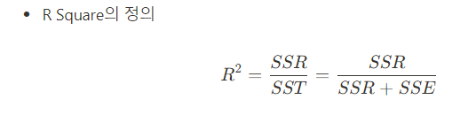
  R Square : 전체 모형에서 회귀선으로 설명할 수 있는 정도
  
  
  

---

📌 선형회귀 실습

---

📌 라이브러리 설치 및 불러오기

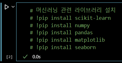
라이브러리 설치

# 머신러닝 관련 라이브러리 설치 (버전에 따라 ! 유무)
!pip install scikit-learn
!pip install numpy
!pip install pandas
!pip install matplotlib
!pip install seaborn

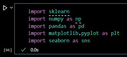
라이브러리 불러오기

import sklearn
import numpy as np
import pandas as pd
import matplotlib.pyplot as plt
import seaborn as sns

---

📌 키 - 몸무게 데이터 실습

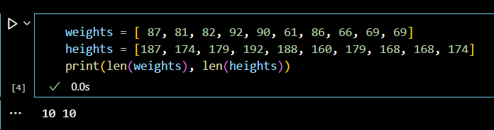
데이터 생성

weights = [ 87, 81, 82, 92, 90, 61, 86, 66, 69, 69]
heights = [187, 174, 179, 192, 188, 160, 179, 168, 168, 174]
print(len(weights), len(heights))

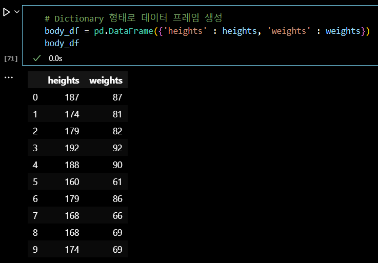
# Dictionary 형태로 데이터 프레임 생성
body_df = pd.DataFrame({'heights' : heights, 'weights' : weights})
body_df

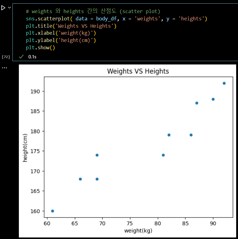
산점도 그리기

# weights 와 heights 간의 산점도 (scatter plot)
sns.scatterplot( data = body_df, x = 'weights', y = 'heights')
plt.title('Weights VS Heights')
plt.xlabel('weight(kg)')
plt.ylabel('height(cm)')
plt.show()

선형회귀 모델 불러오고 훈련하기

# 선형회귀 훈련(train : 적합)
from sklearn.linear_model import LinearRegression
lr = LinearRegression()
type(lr)

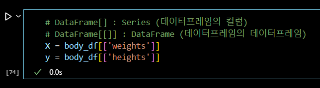
# DataFrame[] : Series (데이터프레임의 컬럼)
# DataFrame[[]] : DataFrame (데이터프레임의 데이터프레임)
X = body_df[['weights']]
y = body_df[['heights']]

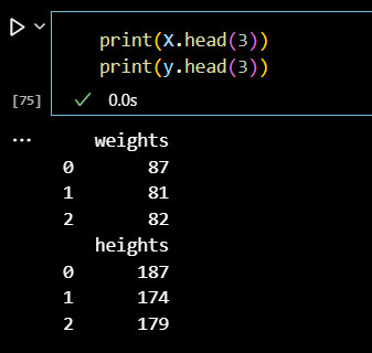
print(X.head(3))
print(y.head(3))

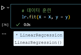
# 데이터 훈련
lr.fit(X = X, y = y)

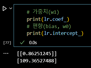
# 가중치(w1)
print(lr.coef_)
# 편향(bias, w0)
print(lr.intercept_)

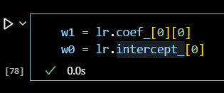
# 변수 생성
w1 = lr.coef_[0][0]
w0 = lr.intercept_[0]

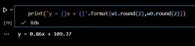
print('y = {}x + {}'.format(w1.round(2),w0.round(2)))
# y = 0.86x + 109.37
# y(heights)는 X(weights)에 0.86을 곱한 뒤 109.37을 더하면 된다.

---

📌 코드 학습 방법

# 1. 구글링 > 블로그
# 장점 : 원하는 내용을 편하게 찾을 수 있다.
# 단점 : 검색 결과가 늘 변하고, 형태가 일정하지 않다.

# 2. ChatGPT - LLM
# 장점 : 편하고 쉽다.
# 단점 : 의존하게 되면 공부를 하지 않고, 거짓된 정보를 전달하는 경우가 있다.

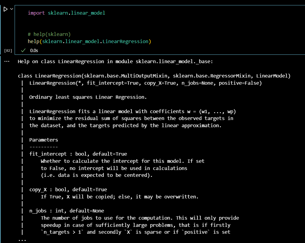
# 3. 공식문서
# 장점 : 일괄된 문서 정리, 동일한 위치(경로)에 같은 문서가 있다.
# 단점 : 초보자가 읽기 어렵다.

import sklearn.linear_model
# help(sklearn)
help(sklearn.linear_model.LinearRegression)

---

📌 선형회귀 평가지표 실습

MSE

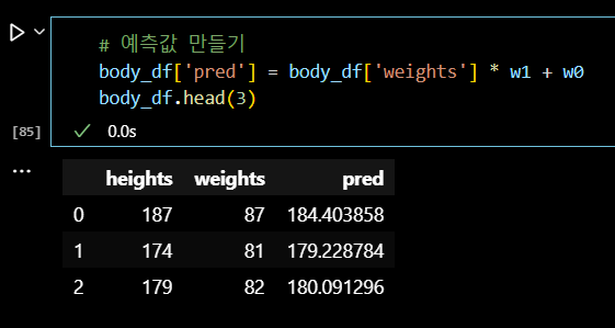
# y = 0.86x + 109.37
# 회귀식을 활용하여 예측 컬럼을 추가
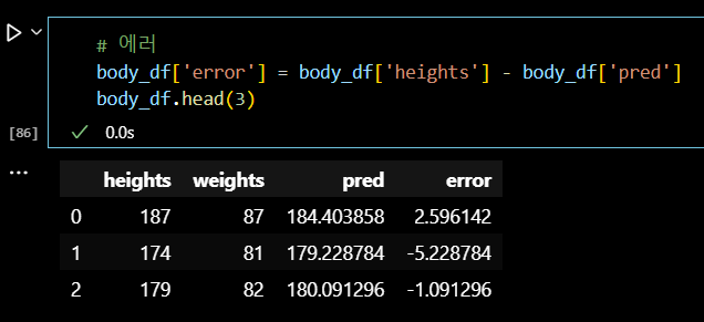
# 에러값을 각각 계산 (error)
# 양수를 만들기 위해 제곱
# 모두 더하면 MSE

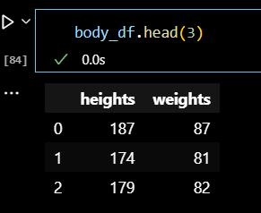
body_df.head(3)

# 예측값 만들기
body_df['pred'] = body_df['weights'] * w1 + w0
body_df.head(3)

# 에러
body_df['error'] = body_df['heights'] - body_df['pred']
body_df.head(3)

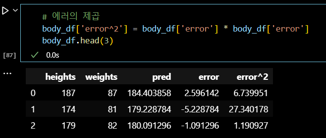
# 에러의 제곱
body_df['error^2'] = body_df['error'] * body_df['error']
body_df.head(3)

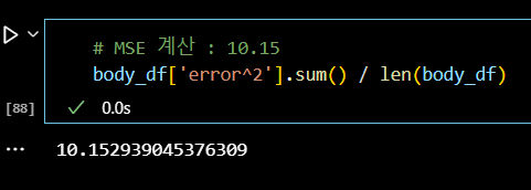
# MSE 계산 : 10.15
body_df['error^2'].sum() / len(body_df)

---

📌 산점도 + 선형식 그래프

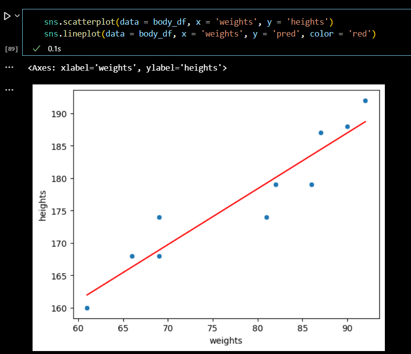
sns.scatterplot(data = body_df, x = 'weights', y = 'heights')
sns.lineplot(data = body_df, x = 'weights', y = 'pred', color = 'red')

---

📌 선형회귀 모델로 예측 & 평가

# 선형회귀 모델 평가
   - 회귀 (숫자를 맞추는 방법) : MSE(수동 계산 결과 = 10)
   - R - Square 값 : 평균 대비 설명력, 0 ~ 1 값, 1일수록 높은 것

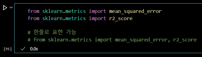
from sklearn.metrics import mean_squared_error
from sklearn.metrics import r2_score
# 한줄로도 표현 가능
# from sklearn.metrics import mean_squared_error, r2_score

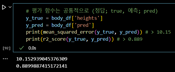
# 평가 함수는 공통적으로 (정답; true, 예측; pred)
y_true = body_df['heights']
y_pred = body_df['pred']
print(mean_squared_error(y_true, y_pred)) # > 10.15
print(r2_score(y_true, y_pred)) # > 0.889 

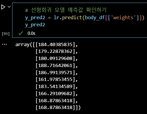
# 선형회귀 모델 예측값 확인하기
y_pred2 = lr.predict(body_df[['weights']])
y_pred2

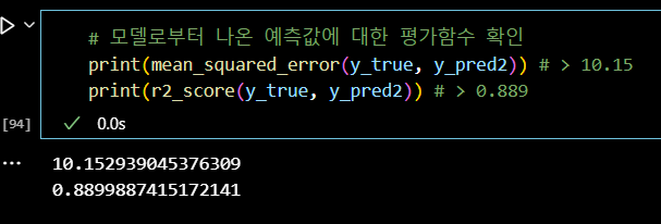
# 모델로부터 나온 예측값에 대한 평가함수 확인
print(mean_squared_error(y_true, y_pred2)) # > 10.15
print(r2_score(y_true, y_pred2)) # > 0.889 

---

📌 tips 데이터 실습

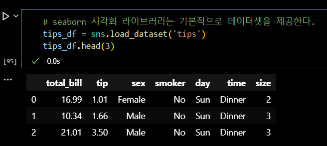
# seaborn 시각화 라이브러리는 기본적으로 데이터셋을 제공한다.
tips_df = sns.load_dataset('tips')
tips_df.head(3)

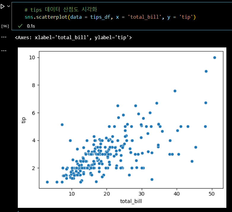
# tips 데이터 산점도 시각화
sns.scatterplot(data = tips_df, x = 'total_bill', y = 'tip')

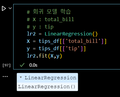
# 회귀 모델 학습
# X : total_bill
# y : tip
lr2 = LinearRegression()
X = tips_df[['total_bill']]
y = tips_df[['tip']]
lr2.fit(X,y)

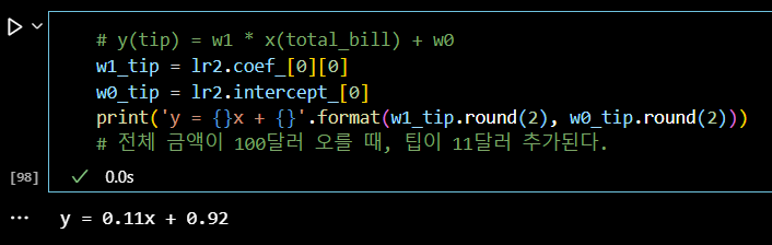
# y(tip) = w1 * x(total_bill) + w0
w1_tip = lr2.coef_[0][0]
w0_tip = lr2.intercept_[0]
print('y = {}x + {}'.format(w1_tip.round(2), w0_tip.round(2)))
# 전체 금액이 100달러 오를 때, 팁이 11달러 추가된다.

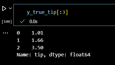
# 예측값 생성
y_true_tip = tips_df['tip']
y_pred_tip = lr2.predict(tips_df[['total_bill']])

y_true_tip[:3]

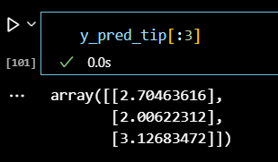
y_pred_tip[:3]

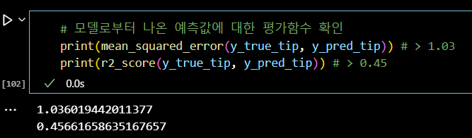
# 모델로부터 나온 예측값에 대한 평가함수 확인
print(mean_squared_error(y_true_tip, y_pred_tip)) # > 1.03
print(r2_score(y_true_tip, y_pred_tip)) # > 0.45 

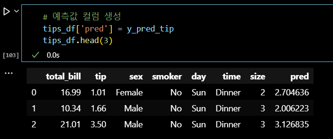
# 예측값 컬럼 생성
tips_df['pred'] = y_pred_tip
tips_df.head(3)

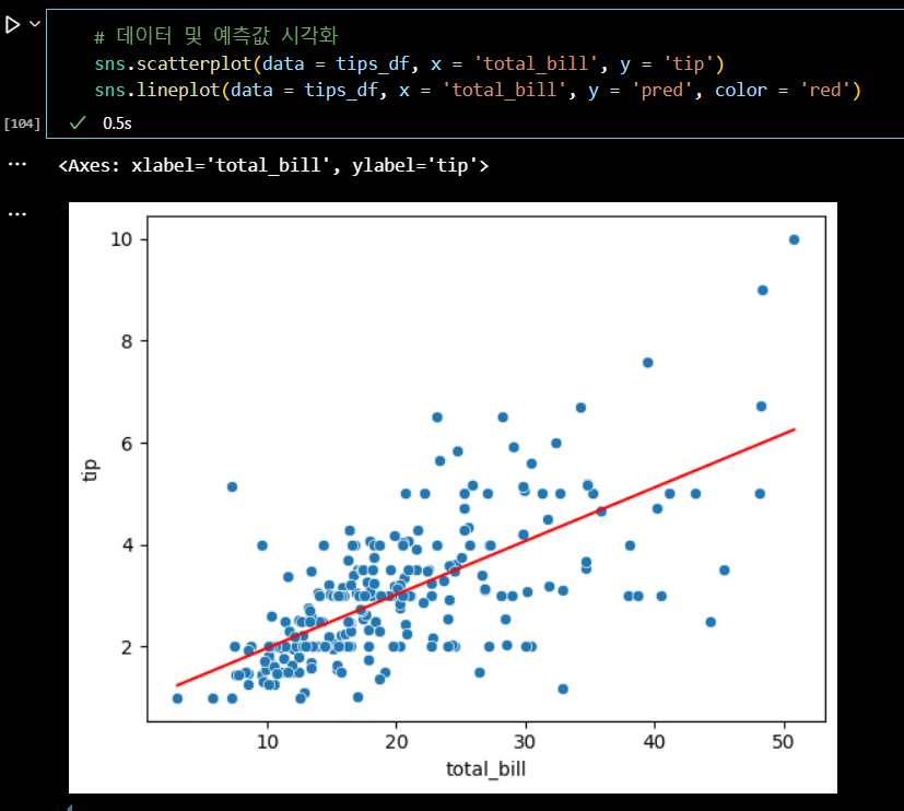
# 데이터 및 예측값 시각화
sns.scatterplot(data = tips_df, x = 'total_bill', y = 'tip')
sns.lineplot(data = tips_df, x = 'total_bill', y = 'pred', color = 'red')

---

📌 선형회귀 심화

• 다중 선형 회귀

단순 선형회귀 vs 다항회귀
범주형 데이터 사용 : 수치형 데이터 vs 범주형 데이터
범주형 데이터를 인코딩하여 회귀 분석이 가능하다.

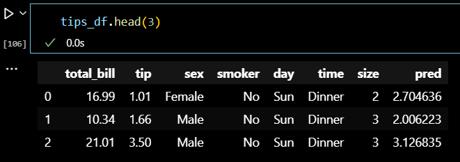
tips_df.head(3)

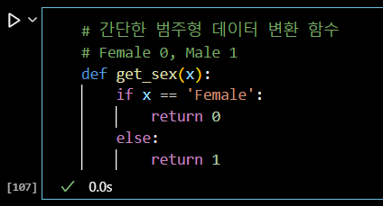
# 간단한 범주형 데이터 변환 함수
# Female 0, Male 1
def get_sex(x):
    if x == 'Female':
        return 0
    else:
        return 1

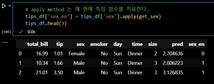
# apply method 는 매 행에 특정 함수를 적용한다.
tips_df['sex_en'] = tips_df['sex'].apply(get_sex)
tips_df.head(3)

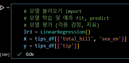
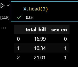
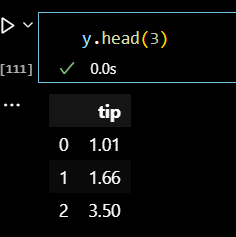
# 모델 불러오기 import
# 모델 학습 및 예측 fit, predict
# 모델 평가 (각종 검정, 지표)
lr3 = LinearRegression()
X = tips_df[['total_bill', 'sex_en']]
y = tips_df[['tip']]

X.head(3)

y.head(3)

lr3.fit(X,y)

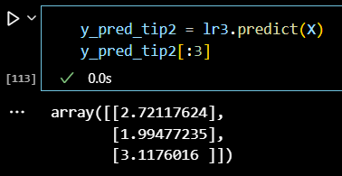
y_pred_tip2 = lr3.predict(X)
y_pred_tip2[:3]

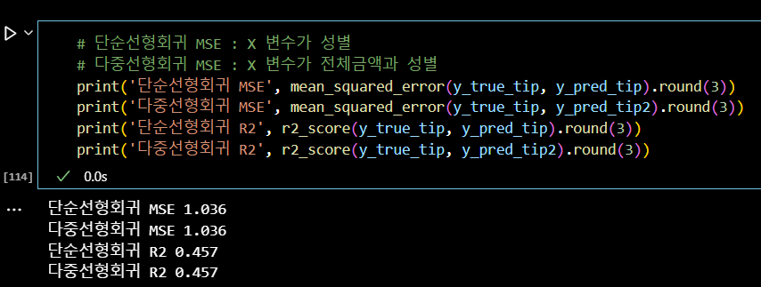
# 단순선형회귀 MSE : X 변수가 성별
# 다중선형회귀 MSE : X 변수가 전체금액과 성별
print('단순선형회귀 MSE', mean_squared_error(y_true_tip, y_pred_tip).round(3))
print('다중선형회귀 MSE', mean_squared_error(y_true_tip, y_pred_tip2).round(3))
print('단순선형회귀 R2', r2_score(y_true_tip, y_pred_tip).round(3))
print('다중선형회귀 R2', r2_score(y_true_tip, y_pred_tip2).round(3))

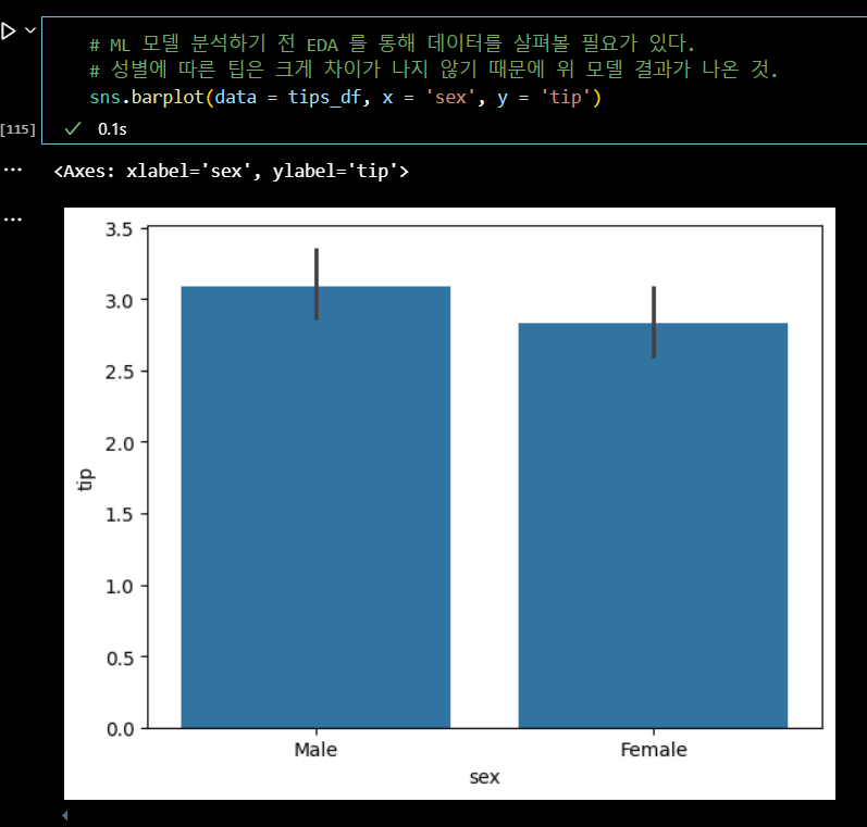
# ML 모델 분석하기 전 EDA 를 통해 데이터를 살펴볼 필요가 있다.
# 성별에 따른 팁은 크게 차이가 나지 않기 때문에 위 모델 결과가 나온 것.
sns.barplot(data = tips_df, x = 'sex', y = 'tip')