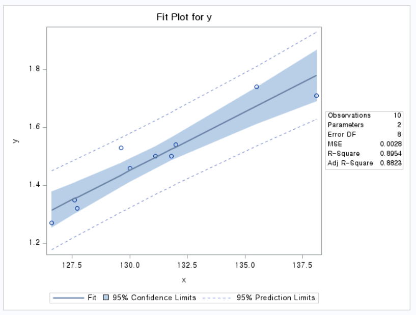
3.1 최대산소흡입량 문제를 다시 고려할 때 (1) 잔차를 구하고 (2) 설명변수 x에 대한 잔차 그림과 반응변수의 예측값 yhat에 대한 잔차그림 그려라.
title 'RESIDUAL PLOT';
data max1;
	input y x;
	lines;
	1.54 132.0
 	1.74 135.5
	1.32 127.7
	1.50 131.1
	1.46 130.0
	1.35 127.6
	1.53 129.6
	1.71 138.1
	1.27 126.6
	1.50 131.8
run;
proc reg data=max1;
 model y=x;
여기서부터 새로운 개념:
output파일 지정, p가 y예측 값, r이 잔차
1. prog reg으로 잔차 plot 확인해서
2. 그에 맞게 vaxis정하기
output out=new p=yhat r=resid;
run;
proc print data=new; /*new로 지정한 앞에 세가지 값들을 print하겠다!*/
run;
symbol v=dot h=0.6;
proc gplot data=new;
plot resid*x / haxis=125 to 140 by 1
				vaxis=-0.1 to 0.1 by 0.01
				vref=0;
plot resid*yhat / haxis=1.2 to 1.8 by 0.1
				   vaxis=-0.1 to 0.1 by 0.01
				   vref=0;
run;
>
이 직선을 조금만 왼쪽으로 꺾으면 아래 그림이 된다! (yref=0으로 선 그음)
3.2 히말라야 산에서 물의 비등점(F)과 압력을 측정하였다. 이 자료에서 물의 비등점을 X로, 압력을 Y로 하여 (1)산점도와 적합선 그리고 (2)스튜던트화 잔차 그림을 그리고 해석하라.
data mountain;
	input x y;
	cards;
	180.6  15.376
	181.0  15.919
	181.9  16.106
	181.9  15.928
	182.4  16.235
	183.2  16.385
	184.1  16.959
	184.1  16.817
	184.6  16.881
	185.6  17.062
	185.7  17.267
	186.0  17.221
	188.5  18.507
	188.8  18.356
	189.5  18.869
	190.6  19.386
	191.1  19.490
	191.4  19.758
	193.4  20.480
	193.6  20.212
	195.6  21.605
	196.3  21.654
	196.4  21.928
	197.0  21.892
	199.5  23.030
	200.1  23.369
	200.6  23.726
	202.5  24.697
	208.4  27.972
	210.2  28.559
	210.8  29.211
run;
1. 스튜던트화 잔차 'student'를 e로 저장(입실론)
proc reg data=mountain;
 model y=x;
 output out=new student=e;
run;
2. i=rl로 x와 y의 산점도랑 회귀선이랑 겹쳐그리기
title scatter plot;
proc gplot data=mountain;
 plot y*x / haxis=175 to 215 by 5
 			vaxis=15 to 30 by 1;
 symbol h=0.5 v=dot, i=rl;
run;
3. 저장했던 'new'를 data로 불러와서 gplot 그리기 (haxis, vaxis는 굳이 안 정해도 되는듯?)
title 'Student Residuals';
proc gplot data=new;
 plot e*x / haxis=175 to 215 by 5
 			vref=0;
 symbol h=0.5 v=dot;
run;
예제 3.3 하드보드 문제에서 설정된 단순회귀모형이 적절한지 '적합결여검정' 해라.
'적합결여검정'(SSPE, SSFL)할 때는 PROC REG 안해도 된다!!!!!
data board;
 input x y;
 cards;
40 66.30
40 64.84
40 64.36
45 69.70
45 66.26
45 72.06
50 73.23
50 71.40
50 68.85
55 75.78
55 72.57
55 76.64
60 78.87
60 77.37
60 75.94
65 78.82
65 77.13
65 77.09
;
run;
proc sort data=board out=sorted;  /* x값에 대해 오름차순으로 정렬*/
 by x;
 run;
 proc print data=sorted;
 run;
title 'LACK-OF-FIT-TEST';
data sorted;
 set sorted;
 retain tempx lack;
 if _n_=1 then do; lack=1;     /*x 변수가 첫 수준일때 lack에 1을 저장 */
	   		 	   tempx=x;
                end;
 else if x=tempx then tempx=x;
 else do; lack=lack+1;    /* x 변수의 수준이 달라지면 lack값이 1 증가*/
	  	  tempx=x;
	  end;
run;
proc print data=sorted;
 var y x tempx lack;
run;
proc glm data=sorted;
 class lack;
 model y= x lack;
run;
proc 'glm'????????
GLM이란?
GLM이란 종속변수 y의 error term이 정규분포가 아닌 다른 분포를 가지는 경우를 포함하는 여러가지 모델들을 아우르는 표현이다. GLM은 Linear Regression, Logistic Regression, Poisson Regression을 포함한다.
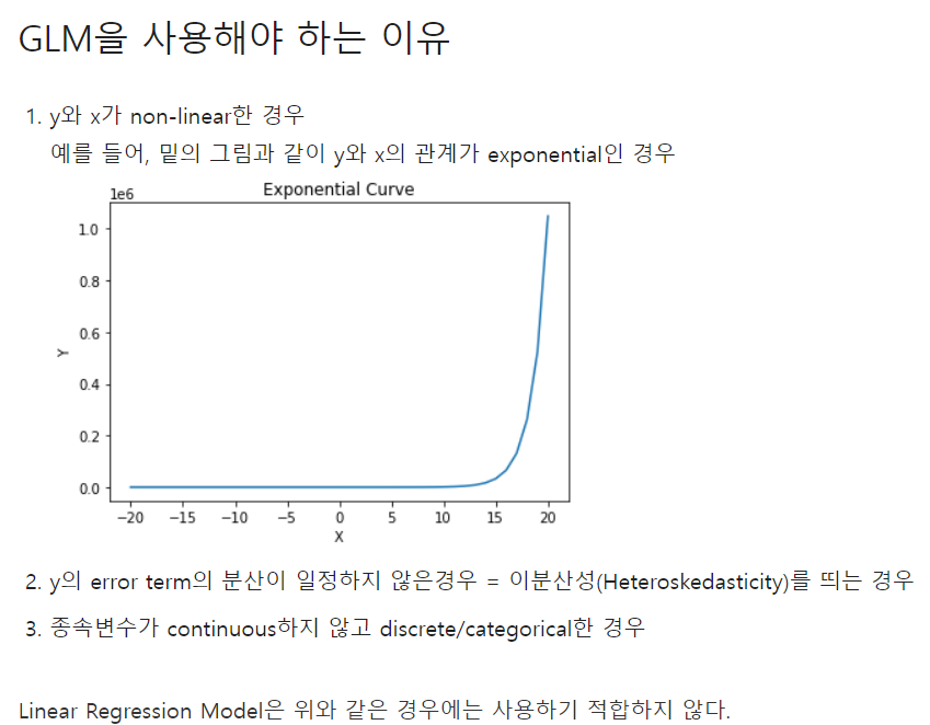
GLM의 model들은 y와 x의 관계가 선형이 아니더라도 'Link Function'을 통해서 선형관계를 만들어 줄 수 있다.
