[ VAE ] 2. code review

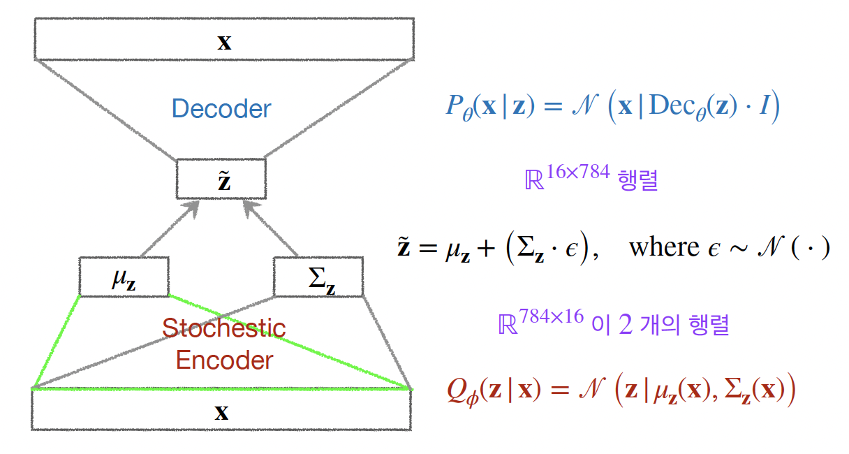
Variational Auto-Encoder (Base-VAE) 코드 구현 및 설명.

import torch
import torch.nn as nn
from torch.nn import functional as F

class Encoder(nn.Module):
    def __init__(self, x_dim, q_dim, z_dim):
        super(Encoder, self).__init__()

        self.x_real = nn.Linear(x_dim, q_dim)
        self.q_hidden = nn.Linear(q_dim, q_dim)
        self.z_mu = nn.Linear(q_dim, z_dim)
        self.z_logvar = nn.Linear(q_dim, z_dim)

        self.q_activation = nn.ReLU()

    def forward(self, x):
        x = self.q_activation(self.x_real(x))
        x = self.q_activation(self.q_hidden(x))
        z_mu = self.z_mu(x)
        z_logvar = self.z_logvar(x)

        return z_mu, z_logvar

class Decoder(nn.Module):
    def __init__(self, z_dim, p_dim, x_dim):
        super(Decoder, self).__init__()

        self.z_real = nn.Linear(z_dim, p_dim)
        self.p_hidden = nn.Linear(p_dim, p_dim)
        self.x_output = nn.Linear(p_dim, x_dim)

        self.p_activation = nn.ReLU()

    def forward(self, x):
        x = self.p_activation(self.z_real(x))
        x = self.p_activation(self.p_hidden(x))
        
        output = torch.sigmoid(self.x_output(x))

        return output

class BaseVAE(nn.Module):
    def __init__(self, Encoder, Decoder):
        super(BaseVAE, self).__init__()
        self.Encoder = Encoder
        self.Decoder = Decoder
       
    def reparameterization(self, z_mu, z_logvar):
        z_var = torch.exp(z_logvar)
        epsilon = torch.randn_like(z_var)

        z = z_mu + torch.sqrt(z_var + 1e-6) * epsilon
        return z
    
    def forward(self, x):
        z_mu, z_logvar = self.Encoder(x)
        z = self.reparameterization(z_mu=z_mu, z_logvar=z_logvar)
        output = self.Decoder(z)

        return output, z_mu, z_logvar

• activation out

  • 최종적으로 decoder 에서 나오는 reconstruct 된 값에 sigmoid 를 사용.

  • mnist 가 흑백 이미지 이므로, pixel 의 값을 0~1 로 quantization 시킬 것.

  • sigmoid 를 거치면, 모든 값이 0~1 로 가게 되면서 원하는 dataspace 와 잘 맞게 된다.

• variable

  • x_real : input

  • x_output : reconstruction term : x_real 과 같은 dimension.

  • z_real : x 상관 없이 latent space 에만 값을 집어 넣어서 sampling 할 때.

• encoder

  • latent space vector 를 만들어줌.

  • stochastic encoder 이므로, latent space 에 대한 분포를 정의.

  • z_mu : 평균 값, z_logvar : variance 가 음수가 되면 안되므로 logvar.

  • neural net 자체는 log-variance 가 나오게 하고, exponential 을 곱해줘서, variance 가 나오게 한다.

  • neural-net 에 어떤 $x$ 가 주어지게 되면, latent space 의 mu, var 이 나온다.

• sampling (reparameterization trick)

  • random dist eps 를 만들고, variance 에 sqrt 시킨것을 곱해서 sampling 을 한것.
  • $x$ 는 고정되어, z_mu, z_var 는 고정, z_sample 은 randomness 때문에 매번 달라짐.
  • 학습에 이런 것을 사용하는 것을 reparameterization trick.

• decoder

  • 이렇게 얻어진 z_sample 이 z_real 로 들어가서 나온 x_output 과 x_real 을 비교.

  • loss 를 줄이는 방향으로 학습하게 된다.

import torch
import torch.nn as nn
import torch.optim as optim
import tqdm

class Train:
    def __init__(self, epochs):
        self.epochs = epochs

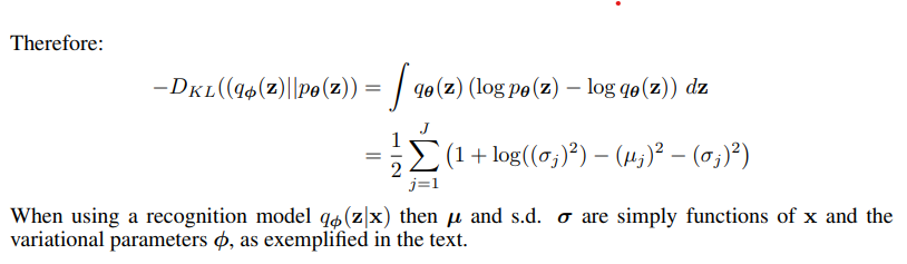
    def loss_func(self, x, output, z_mu, z_logvar):
        reconstruction_loss = nn.functional.binary_cross_entropy(
            input=output,
            target=x,
            reduction='sum'
        )
        kld_loss = -0.5 * torch.sum(1 + z_logvar - z_mu.pow(2) - z_logvar.exp())

        return reconstruction_loss + kld_loss

    def training(self,
                 device,
                 model,
                 data_train,
                 h_param: dict):
        
        print(h_param)
        optimizer = optim.Adam(
                        model.parameters(),
                        lr=h_param["learning_rate"]
                    )
        
        for epoch in range(self.epochs):
            model.train()

            # train
            train_progress = tqdm.tqdm(iterable=data_train
                                    , bar_format="{l_bar}{bar:25}{r_bar}"
                                    , colour="green"
                                    , total=len(data_train)
                                    , leave=True)
            data_size = 0
            train_loss = 0.0
            train_loss_sum = 0.0
            
            for tr_data, _ in train_progress:

                x = tr_data.view(h_param["batch_size"], h_param["x_dim"])
                x = x.to(device)

                # forward
                output, z_mu, z_logvar = model(x)
                train_loss = self.loss_func(x=x,
                                      output=output,
                                      z_mu=z_mu,
                                      z_logvar=z_logvar)
                # backward
                optimizer.zero_grad()
                train_loss.backward()

                train_loss_sum += train_loss.item()
                
                # gradient descent or optimizer step
                optimizer.step()
                
                data_size += len(tr_data)
                train_loss_avg = train_loss_sum / data_size

                # update progress bar
                train_progress.set_description(f"train [{epoch + 1}/{self.epochs}]")
                str_train_loss = '{:.6f}'.format(round(train_loss_avg, 6))
                train_progress.set_postfix(loss=str_train_loss)

        torch.save(model.state_dict(), "/home/d4r6j/ViT_pilot/model/VAE/mnise_vae.pt")

        return model

• loss

  • loss 는 L1, L2 등을 design 해서 사용해도 된다.

  • 여기서는 sigmoid 로 linear 에서 0, 1 로 나온 vector 를 가지고, binary_cross_entropy (BCE) 를 사용.

  • kld loss

    • kld_loss = -0.5 * torch.sum(1 + z_logvar - z_mu.pow(2) - z_logvar.exp())

    • vae paper appendix : Solution of $−D_{KL}(q_{\phi}(z)||p_{\theta}(z))$, Gaussian case 참고.

  • bce loss + (beta) kld loss 를 합쳐서 loss 를 사용한다.

• logvar

  • layer 학습 시, 음수가 나올 수 있으므로 $\sigma$ (표준편차) 값이 음수가 되지 않도록 logvar 로 정한다.

from torchvision import datasets
import torchvision.transforms as transforms
from torch.utils.data import DataLoader

import torch

device = torch.device("cuda" if torch.cuda.is_available() else "cpu")
data_path = "/data/images/mnist"

H_PARAM = [
    {
        "x_dim": 784,
        "h_dim": 256,
        "z_dim": 16,
        "learning_rate": 1e-3,
        "batch_size": 50
    }
]

# ----------------------------------------------------------------
#         Layer (type)               Output Shape         Param #
# ================================================================
#             Linear-1               [-1, 1, 256]         200,960
#               ReLU-2               [-1, 1, 256]               0
#             Linear-3               [-1, 1, 256]          65,792
#               ReLU-4               [-1, 1, 256]               0
#             Linear-5                [-1, 1, 16]           4,112
#             Linear-6                [-1, 1, 16]           4,112
#            Encoder-7  [[-1, 1, 16], [-1, 1, 16]]               0
#             Linear-8               [-1, 1, 256]           4,352
#               ReLU-9               [-1, 1, 256]               0
#            Linear-10               [-1, 1, 256]          65,792
#              ReLU-11               [-1, 1, 256]               0
#            Linear-12               [-1, 1, 784]         201,488
#           Decoder-13               [-1, 1, 784]               0
# ================================================================
# Total params: 546,608
# Trainable params: 546,608
# Non-trainable params: 0
# ----------------------------------------------------------------
# Input size (MB): 0.00
# Forward/backward pass size (MB): 0.03
# Params size (MB): 2.09
# Estimated Total Size (MB): 2.11
# ----------------------------------------------------------------

def main(h_param, epochs):

    train = Train(
        epochs=epochs
    )

    for i in range(len(h_param)):
        encoder = Encoder(x_dim=H_PARAM[i]["x_dim"],
                          q_dim=H_PARAM[i]["h_dim"],
                          z_dim=H_PARAM[i]["z_dim"])
        
        decoder = Decoder(z_dim=H_PARAM[i]["z_dim"],
                          p_dim=H_PARAM[i]["h_dim"],
                          x_dim=H_PARAM[i]["x_dim"])

        model = BaseVAE(Encoder=encoder, Decoder=decoder).to(device)

        transform = transforms.Compose([
                transforms.ToTensor(),
        ])

        tr_dataset = datasets.MNIST(root=data_path,
            train=True,
            download=True,
            transform=transform
        )

        te_dataset = datasets.MNIST(root=data_path,
            train=False,
            download=True,
            transform=transform
        )

        data_train = DataLoader(dataset=tr_dataset,
                                batch_size=h_param[i]["batch_size"],
                                shuffle=True)
        data_test  = DataLoader(dataset=te_dataset,
                                  batch_size=h_param[i]["batch_size"],
                                  shuffle=False)
        trained_model = train.training(device=device,
                       model=model,
                       data_train=data_train,
                       h_param=h_param[i])
    
    return trained_model

trained_model = main(h_param=H_PARAM, epochs=60)

{'x_dim': 784, 'h_dim': 256, 'z_dim': 16, 'learning_rate': 0.001, 'batch_size': 50}
train [1/60]: 100%|█████████████████████████| 1200/1200 [00:05<00:00, 219.89it/s, loss=158.840946]
train [2/60]: 100%|█████████████████████████| 1200/1200 [00:05<00:00, 205.21it/s, loss=121.427494]
train [3/60]: 100%|█████████████████████████| 1200/1200 [00:05<00:00, 208.10it/s, loss=114.462988]
train [4/60]: 100%|█████████████████████████| 1200/1200 [00:05<00:00, 209.38it/s, loss=111.280789]
train [5/60]: 100%|█████████████████████████| 1200/1200 [00:05<00:00, 212.91it/s, loss=109.441187]
train [6/60]: 100%|█████████████████████████| 1200/1200 [00:05<00:00, 212.64it/s, loss=108.119385]
train [7/60]: 100%|█████████████████████████| 1200/1200 [00:05<00:00, 202.08it/s, loss=107.181680]
train [8/60]: 100%|█████████████████████████| 1200/1200 [00:05<00:00, 203.34it/s, loss=106.438379]
train [9/60]: 100%|█████████████████████████| 1200/1200 [00:05<00:00, 209.44it/s, loss=105.831416]
train [10/60]: 100%|█████████████████████████| 1200/1200 [00:05<00:00, 201.01it/s, loss=105.304058]
train [11/60]: 100%|█████████████████████████| 1200/1200 [00:05<00:00, 209.12it/s, loss=104.858765]
train [12/60]: 100%|█████████████████████████| 1200/1200 [00:05<00:00, 206.99it/s, loss=104.492835]
train [13/60]: 100%|█████████████████████████| 1200/1200 [00:05<00:00, 212.22it/s, loss=104.114048]
train [14/60]: 100%|█████████████████████████| 1200/1200 [00:05<00:00, 203.28it/s, loss=103.850844]
train [15/60]: 100%|█████████████████████████| 1200/1200 [00:05<00:00, 206.18it/s, loss=103.520258]
train [16/60]: 100%|█████████████████████████| 1200/1200 [00:05<00:00, 209.32it/s, loss=103.332970]
train [17/60]: 100%|█████████████████████████| 1200/1200 [00:05<00:00, 203.38it/s, loss=103.104726]
train [18/60]: 100%|█████████████████████████| 1200/1200 [00:06<00:00, 195.52it/s, loss=102.861201]
train [19/60]: 100%|█████████████████████████| 1200/1200 [00:05<00:00, 204.39it/s, loss=102.684826]
train [20/60]: 100%|█████████████████████████| 1200/1200 [00:05<00:00, 201.12it/s, loss=102.473160]
train [21/60]: 100%|█████████████████████████| 1200/1200 [00:06<00:00, 197.14it/s, loss=102.327501]
train [22/60]: 100%|█████████████████████████| 1200/1200 [00:06<00:00, 192.86it/s, loss=102.172790]
train [23/60]: 100%|█████████████████████████| 1200/1200 [00:05<00:00, 202.85it/s, loss=102.052731]
train [24/60]: 100%|█████████████████████████| 1200/1200 [00:05<00:00, 200.28it/s, loss=101.863789]
train [25/60]: 100%|█████████████████████████| 1200/1200 [00:06<00:00, 193.36it/s, loss=101.678621]
...
train [57/60]: 100%|█████████████████████████| 1200/1200 [00:06<00:00, 172.31it/s, loss=99.551849]
train [58/60]: 100%|█████████████████████████| 1200/1200 [00:07<00:00, 168.74it/s, loss=99.567466]
train [59/60]: 100%|█████████████████████████| 1200/1200 [00:06<00:00, 171.84it/s, loss=99.512373]
train [60/60]: 100%|█████████████████████████| 1200/1200 [00:07<00:00, 167.01it/s, loss=99.417055]
Output is truncated. View as a scrollable element or open in a text editor. Adjust cell output settings...

• x_dim : Original data space : 784 ( mnist 28 x 28 흑백 )

• z_dim : Latent space dimension : 현재는 16 차원

  • Latent space 를 직접 plot 하기 위해서는 2 ~ 3 dim 으로 한다.

• VAE netork design plan.

  • encoder (Q)

    • 784 -> 256 -> 256 -> 16

  • decoder (P)

    • 16 -> 256 -> 256 -> 784

  • activation function : ReLU 를 사용. (다른 것을 사용해도 무방)

• betaVAE

  • VAE : reconstruction term 과 prior fitting term : KL-Divergence.

  • KL-Divergence 에 constant (beta) 를 곱하여 hyper-parameter 를 추가.

import matplotlib.pyplot as plt

batch_size = 50
x_dim = 784

transform = transforms.Compose([
                transforms.ToTensor(),
        ])

te_dataset = datasets.MNIST(root=data_path,
            train=False,
            download=True,
            transform=transform
        )

trained_model.eval()
data_test  = DataLoader(dataset=te_dataset,
                            batch_size=batch_size,
                            shuffle=False)
with torch.no_grad():
    for x, _ in data_test:
        x = x.view(batch_size, x_dim)
        x = x.to(device)
        
        x_dec, _, _ = trained_model(x)
        break

x = x.view(batch_size, 28, 28)
x_dec = x_dec.view(batch_size, 28, 28)

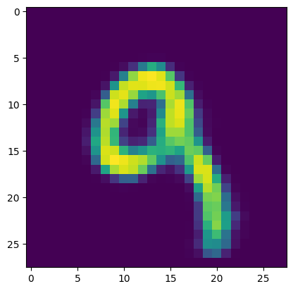
plt.imshow(x[7].cpu().numpy())
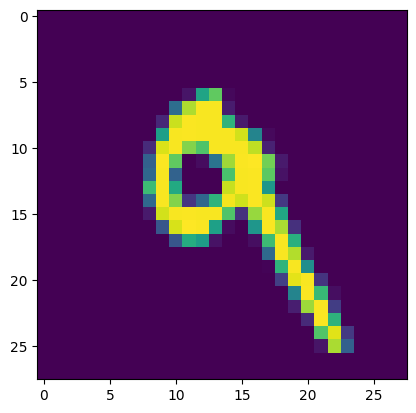
fig = plt.figure()
plt.imshow(x_dec[7].cpu().numpy())

• x_real
  

• z_real