Abstract
문서 레이아웃 분석 ( DLA : Document Layout Analysis ) 는 실제 문서 이해 시스템에서 매우 핵심적이지만, 속도와 정확도 사이의 trade-off 도전에 직면하게 된다. text 와 visual 기능들을 모두 활용하는 multimodal 방법은 더 높은 정확도를 달성하지만, 상당한 latency 가 발생하는 반면, 시각적인 기능에만 의존하는 unimodal 방법은 처리 속도는 빠르지만 정확도가 떨어진다. 이러한 dilemma 를 해결하기 위해서 pre-training 과 model 설계 모두 document-specific 최적화를 통해서 속도의 잇점은 유지하면서 정확성을 강화하는 새로운 접근 방식인 DocLayout-YOLO 를 소개한다.
Mesh-candidate BsetFit 알고리즘은 문서 내 텍스트, 이미지, 표 등과 같은 문서의 다양한 요소들을 문서 레이아웃에 배치하여 문서를 생성하는 것을 2차원 빈 패킹 (2D bin-packing) 문제로 간주하고 최적의 배치를 찾는다. 이를 통해서 대규모 합성 문서 데이터셋인 DocSynth-300K 가 생성되었으며, 이 데이터 셋은 다양한 문서 레이아웃을 학습하는데 사용한다.
DocSynth300K dataset 에 대한 Pre-training 은 다양한 문서 유형 전반에 걸쳐서 fine-tuning 성능을 크게 향상 시킨다. 모델 최적화의 측면에서는 문서 element 들의 multi-scale 변형을 더욱 잘 핸들링 할 수 있는 Global-to-Local Controllable Receptive Module G2L_CRM 을 제안한다.
무엇보다도 다양한 문서 유형의 성능을 검증하기 위해 DocStructBench 라는 복잡하고 까다로운 벤치마크를 도입했다. 다운스트림 dataset 에 대한 대규모 실험을 통해서 DocLayout-YOLO 는 속도와 정확성 모두 뛰어났다.
Diverse DocSynth-300K dataset construction
기존의 unimodal 사전 훈련 데이터셋은 주로 학술 논문들로 구성되어 상당한 homogeneity 를 특징으로 한다. 이러한 제한은 사전 훈련된 모델의 일반화 기능을 대체적으로 방해한다. 다양한 downstream 문서 유형에 대한 적응력을 높이려면, 보다 다양한 pre-training 문서 dataset 으로 개발하는 것이 필수적이다.
사전 훈련 데이터의 다양성은 주로 두 가지 차원으로 나타날 수 있다.
-
Element diversity
다양한 글꼴 크기의 텍스트, 다양한 형식의 표 등과 같은 다양한 문서 요소가 포함된다.
-
Layout diversity
single-column, double-column, multi-column 을 포함한 다양한 문서 레이아웃과 학술 논문, 잡지 및 신문에 특정한 형식이 포함된다.
element 와 layout 의 다양성을 활용하여 다양하고 잘 구성된 문서를 자동적으로 합성하는 Mesh-candidate BsetFit 이라는 방법론을 제안한다.
Mesh-candidate BestFit

이 결과로 만들어진 DocSynth-300K 데이터셋은 다양한 실제 문서 유형에 걸쳐서 모델 성능을 크게 강화시킨다. Mesh-candidate BestFit 의 전체 파이프라인은 아래에 자세히 설명 되어 있다.
Preprocessing
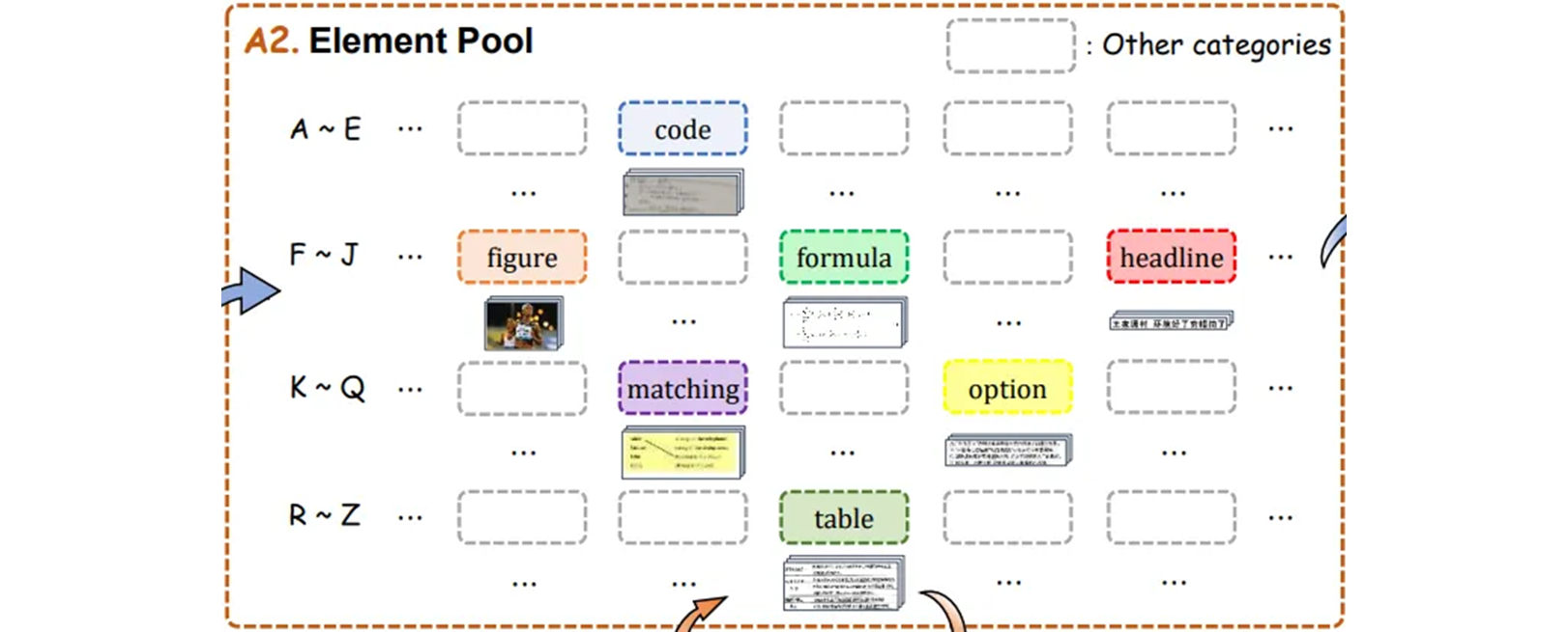
Ensuring element diversity
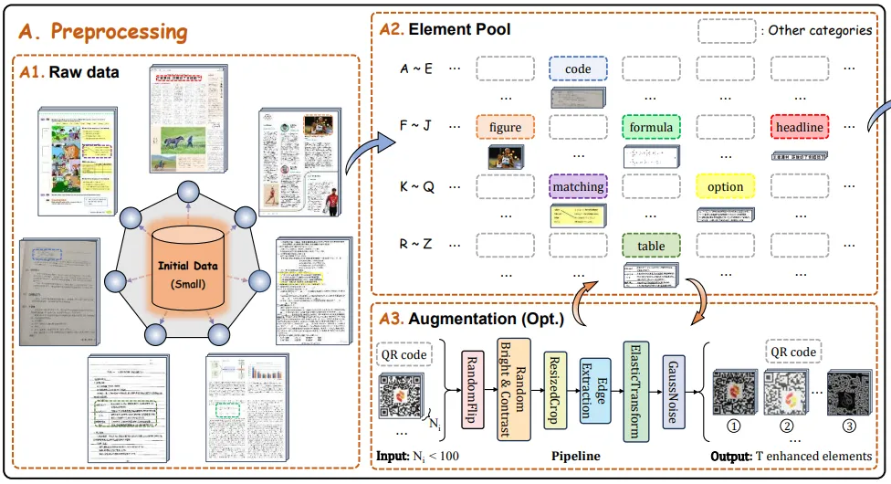
a category-wise element pool is created from a small initial dataset.
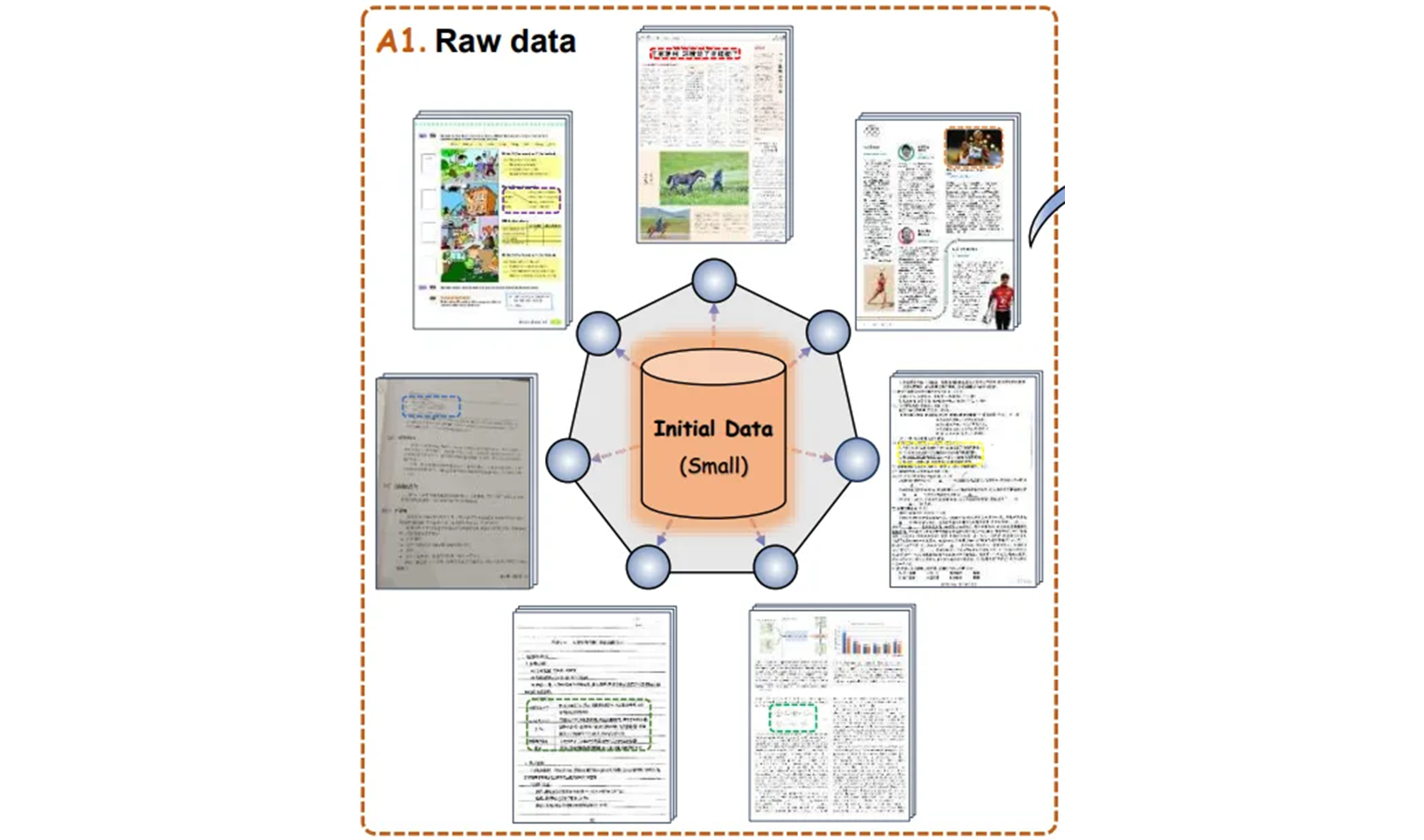
전 처리 단계에서 다양한 범위의 문서 요소들이 포함되도록 보장하기 위해서, 초기 데이터로써 약 2800 개의 다양한 문서 페이지로부터 나오는 74개의 서로 다른 문서 요소로 구성되어 있는 text 를 활용한다.
결과적으로 우리는 페이지를 조각화 하여 각기 세분화된 카테고리별로 element pool 을 추출하고 구성한다. 동일한 카테고리의 요소 내에 다양성을 유지하기 위해서 100 개 미만의 수량을 갖고 있는 희귀 카테고리들의 데이터 pool 을 확장하는 augmentation 파이프라인을 설계한다.
Data preparation
-
annotation file
-
COCO format 을 따르며, JSON file 에는 image 와 instance annotation 이 포함되어 있다.
-
각 instance 에는 고유한 instance_id 가 있어야 한다.
{"id": 16033, "image_id": 635, "category_id": 53, "segmentation": [[638.672131147541, 113.39344262295083, 1117.360655737705, 113.39344262295083, 1117.360655737705, 524.8688524590164, 638.672131147541, 524.8688524590164]], "area": 197760.0, "bbox": [638.0, 113.0, 480.0, 412.0], "iscrowd": 0},

{"id": 16034, "image_id": 635, "category_id": 48, "segmentation": [[604.2459016393443, 1513.393442622951, 622.2786885245903, 1513.393442622951, 622.2786885245903, 1536.344262295082, 604.2459016393443, 1536.344262295082]], "area": 456.0, "bbox": [604.0, 1513.0, 19.0, 24.0], "iscrowd": 0},

{"id": 16035, "image_id": 636, "category_id": 58, "segmentation": [[85.71428571428571, 99.2063492063492, 203.96825396825398, 99.2063492063492, 203.96825396825398, 124.60317460317461, 85.71428571428571, 124.60317460317461]], "area": 3094.0, "bbox": [85.0, 99.0, 119.0, 26.0], "iscrowd": 0},

{"id": 16036, "image_id": 636, "category_id": 53, "segmentation": [[85.0, 129.0, 600.0, 129.0, 600.0, 1476.0, 85.0, 1476.0]], "area": 695568.0, "bbox": [85.0, 129.0, 516.0, 1348.0], "iscrowd": 0}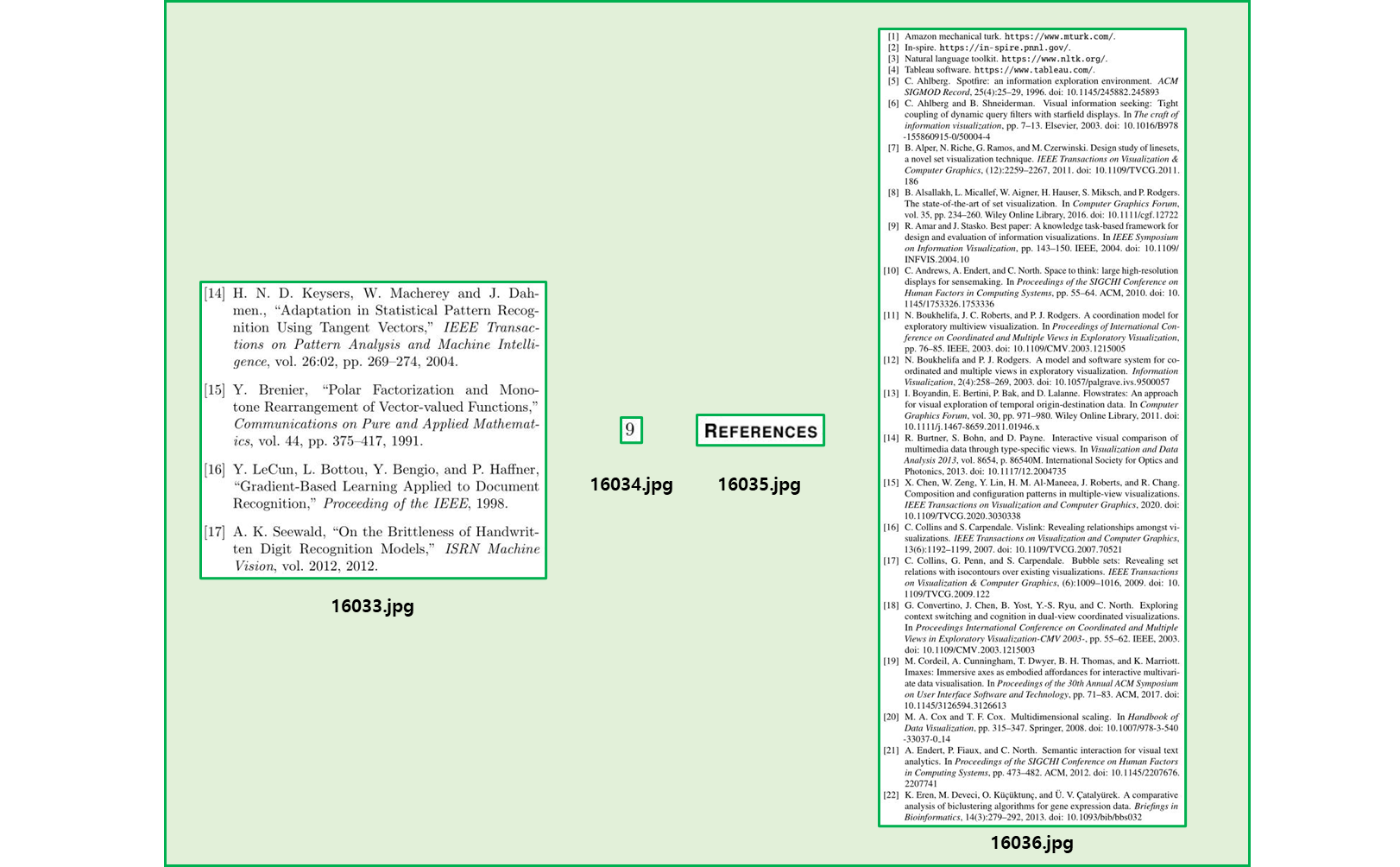
-
-
Element Pool
-
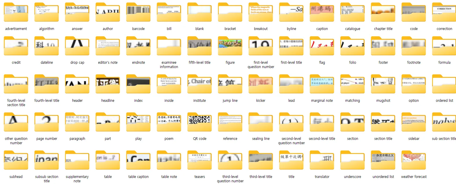
모든 instance image 를 자르고 category 별로 정리한다.
-
-
Data augmentation
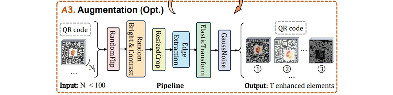
전처리 단계에서 element pool 에 element 가 거의 없는 rare 카테고리에 대해서 특별히 설계된 augmentation pipeline 을 수행한다.
-
Random Flip
다양한 문서에서 텍스트 방향의 다양한 가능성을 고려하여 0.5의 확률로 가로 와 세로 방향으로 random flip 하여 원본 데이터를 강화 한다. -
Random Brightness&Contrast
0.5 의 확률로 element 의 밝기와 대비를 random 하게 바꾸면서 다양한 조명 조건과 밝기 level 에서 실제 환경을 시뮬레이션 한다. -
Random Cropping
model 이 local feature 에 더 집중하도록 가이드하기 위해서 0.7 확률을 사용하여 0.5 ~ 0.9 영역 범위 내의 element 들에 대해 random cropping 을 수행한다. -
Edge Extraction
Sobel filter 를 사용하여 edge detection 을 수행하고 element 내에 contour 정보를 0.2 확률로 추출하여 feature 의 풍부함을 향상 시켰다. -
Elastic Transformation&Gaussian Noisification
reality 에서 jitter 나 resolution (해상도) 로 인한 왜곡을 simulate 하기 위해 약간의elastic transformation과Gaussian noise추가 프로세스를 통해서 원본 데이터를 왜곡하고 흐리게 한다.len(os.listdir(category_dir)) > args.min_countmin_count기준으로 ( default : 100 ) 이면 Augmentation 을 한다.def pipeline(h, w): """ Whole data augmentation pipeline with the input of image size Args: h (float): Height of the image. w (float): Width of the image. """ return A.Compose([ A.RandomBrightnessContrast(p=0.5), A.RandomResizedCrop(height=h, width=w, scale=(0.5, 0.9), ratio=(w / h, w / h), p=0.7), # keep h/w ratio the same EdgeDetection(p=0.2), A.ElasticTransform(alpha_affine=5, p=0.2), A.GaussNoise(var_limit=(100, 1200), p=1), ])
-
실제는
RandomFlip이 없다. 아무래도 document 다 보니Flip을 넣는건 무리가 있었을듯. -
GaussNoise 는 probability 가 1 로 무조건 넣는건 재미난 수치다.
-
-
Map Dict
랜더링 단계에서 candidate 의 무작위 선택을 가능하게 하려면, candidate 요소에서 그들의 모든 경로의 mapping 을 설정해야 한다.
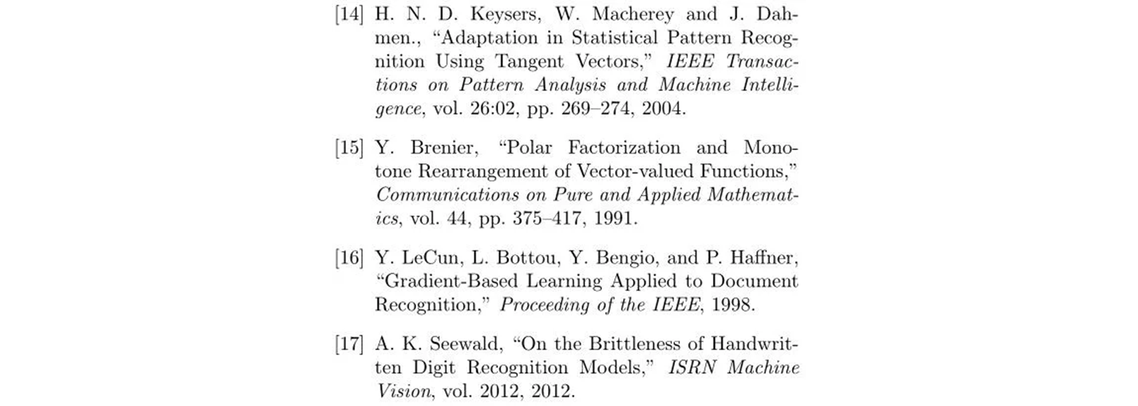
{"10643": ["./element_pool\\advertisement\\10643.jpg"],
 "10848": ["./element_pool\\advertisement\\10848.jpg"],
 "11656": ["./element_pool\\advertisement\\11656.jpg"],
 ...
 "16033": ["./element_pool\\reference\\16033.jpg",
           "./element_pool\\reference\\aug/16033\\16033_1735144650_2257504.jpg",
           "./element_pool\\reference\\aug/16033\\16033_1735144650_2414556.jpg",
           "./element_pool\\reference\\aug/16033\\16033_1735144650_2580667.jpg",
           ...
           "./element_pool\\reference\\aug/16033\\16033_1735144650_3499408.jpg",
           "./element_pool\\reference\\aug/16033\\16033_1735144650_3690825.jpg"]
  ...}
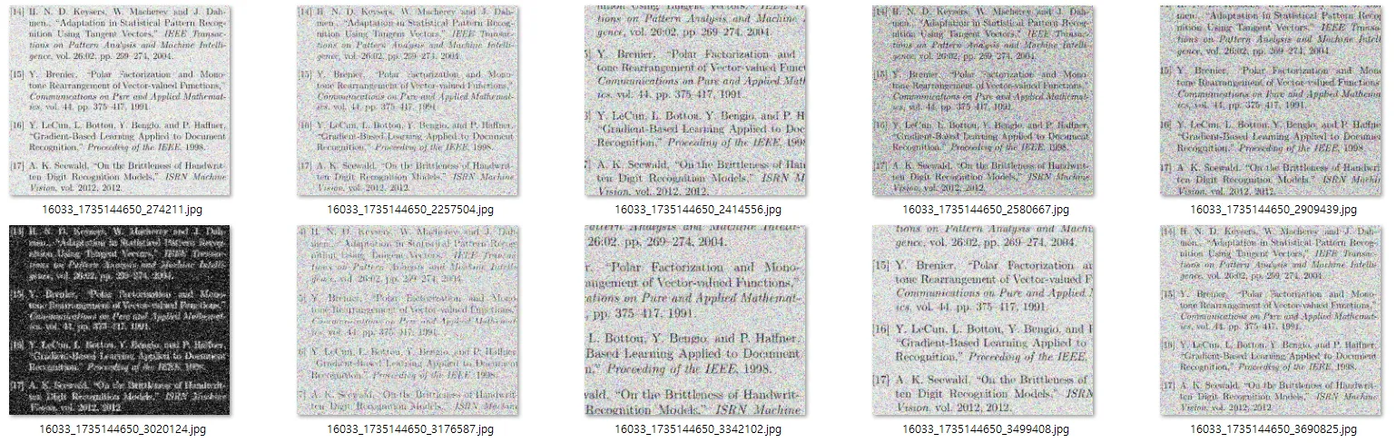
layout generation
ensuring layout diversity
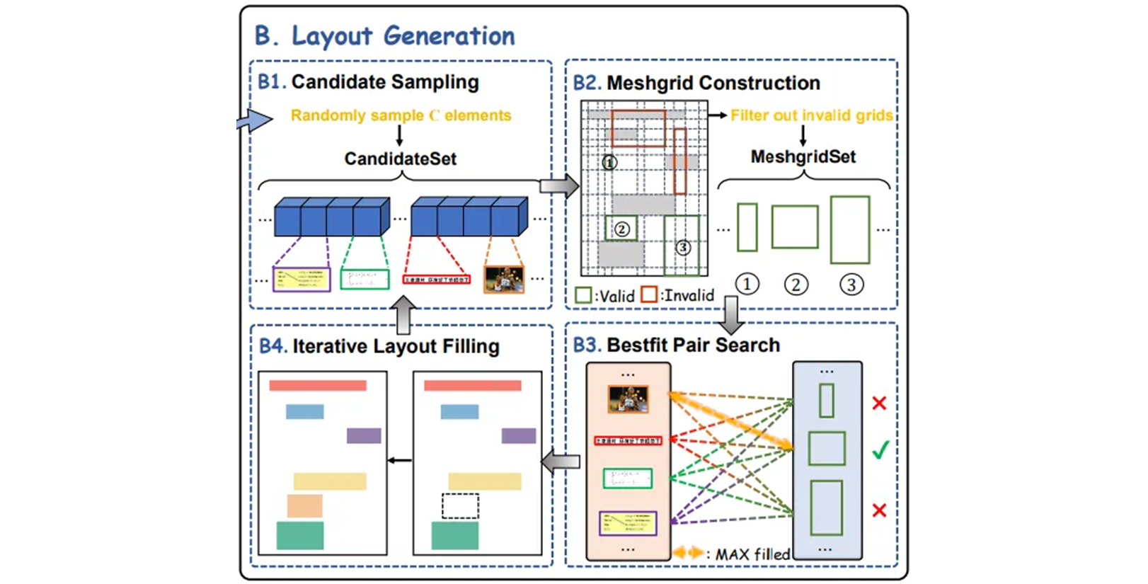
candidate 와 grids (bins) 사이에서 가장 일치하는 항목을 반복적으로 검색한다. 가장 잘 일치하는 쌍을 찾은 후에 candidate 는 문서에 들어가고 element 수가 threshold ( 경험적으로 15 로 설정 됨 ) 에 도달할 때 까지 최적의 매칭을 반복적으로 검색한다. matching threshold 은 로 설정한다.
layout generation 단계에서 size 요구 사항을 충족하는 유효한 쌍이 없을 때 까지 가장 잘 채워진 candidate grid 쌍을 검색하기 위해 최적의 매칭을 반복적으로 수행한다. 또한 작은 element 의 수가 과잉 상태면, 기존의 미적 기준을 따르지 않는 layout 이 되기 때문에 작은 element 의 수가 을 초과 해서는 안된다는 추가적인 제약사항을 추가한다. 특히 은 로 설정한다.
은 각각 소형, 중형, 대형 element 들을 나타내고, page 에서 상대적으로 풍부한 구성 요소를 나타낸다. 생성되는 데이터는 카테고리가 풍부하고 강한 다양성을 갖고 있다는 것이 분명하다. 많은 작은 요소들을 포함하는 dense layout 을 생성할 수 있을 뿐 아니라 diffusion 기반 모델에서 생성된 layout 과 유사하게 몇 개의 큰 element 들로 구성된 sparse layout 도 생성할 수 있다.
# Default candidate_num = 500
candidate_num = 500
large_elements_idx = random.sample(list(range(len(element_all['large']))), int(candidate_num*0.99))
small_elements_idx = random.sample(list(range(len(element_all['small']))), int(candidate_num*0.01))
cand_elements = [element_all['large'][large_idx] for large_idx in large_elements_idx] + [element_all['small'][small_idx] for small_idx in small_elements_idx]
if maxfit_element.w < 0.05 or maxfit_element.h < 0.05:
small_cnt += 1
if small_cnt > 5:
break- Layout Generation
Mesh-candidate BestFit iteratively searches for the optimal candidate-grid match.
다양한 layout 들을 합성하는 문제를 해결하는 데 있어서 가장 쉬운 접근 방식은 무작위 배열이다. 그러나 무작위 배열은 무질서하고 혼란스러운 레이아웃을 생성하여 실제 문서의 개선을 심각하게 방해한다. Diffusion 또는 GAN 기반의 layout 생성 모델과 관련하여 기존 방법은 학술 논문과 같은 동질적인 레이아웃을 생성하는 것으로 다양한 실제 문서 레이아웃을 cover 하기에는 불충분하다.
“2D bin packing” 문제에서 영감을 받아 실제 문서들의 layout 다양성과 일관성을 보장하기 위해서, 현재 layout 으로 만들어진 사용 가능한 grid 를 다양한 크기의 “bins” 으로 보고, 반복적으로 최상의 매칭을 수행하여 layout 의 다양성 (randomness) 과 미적 (fill rate and alignment : 화면 공간, 페이지 요소들이 효율적으로 배치되고 채워지고, 정렬되는지) 부분의 균형을 맞춰서 보다 다양하고 합리적인 document layouts 을 생성한다. layout 생성의 자세한 step 들은 아래와 같다.
Candidate Sampling
각 빈 페이지에 대해 element 크기를 기준으로 element pool 에서 계층화된 샘플링을 통해서 하위 집합을 얻어서 candidate set 으로 사용된다. 그리고 후보 set 에서 element 를 random 하게 샘플링하여 페이지의 특정 위치에 배치한다.

# Initially, randomly put an element
put_elements = []
e0 = random.choice(cand_elements)
cx = random.uniform(min(e0.w/2, 1-e0.w/2), max(e0.w/2, 1-e0.w/2))
cy = random.uniform(min(e0.h/2, 1-e0.h/2), max(e0.h/2, 1-e0.h/2))
e0.cx, e0.cy = cx, cy
put_elements = [e0]
cand_elements.remove(e0)
small_cnt = 1 if e0.w < 0.05 or e0.h < 0.05 else 0Meshgrid Construction

layout 기반으로 meshgrid 를 구성하고
# Construct meshgrid based on current layout
put_element_boxes = []
xticks, yticks = [0,1], [0,1]
for e in put_elements:
x1, y1, x2, y2 = e.cx-e.w/2, e.cy-e.h/2, e.cx+e.w/2, e.cy+e.h/2
xticks.append(x1)
xticks.append(x2)
yticks.append(y1)
yticks.append(y2)
put_element_boxes.append([x1, y1, x2, y2])
xticks, yticks = list(set(xticks)), list(set(yticks))
pticks = list(itertools.product(xticks, yticks))
meshgrid = list(itertools.product(pticks, pticks))
put_element_boxes = torch.Tensor(put_element_boxes)삽입된 요소와 겹치는 잘못된 grid 를 필터링한다.
# Filter out invlid grids
meshgrid = [grid for grid in meshgrid if grid[0][0] < grid[1][0] and grid[0][1] < grid[1][1]]
meshgrid_tensor = torch.Tensor([p1 + p2 for p1, p2 in meshgrid])
iou_res = torchvision.ops.box_iou(meshgrid_tensor, put_element_boxes)
valid_grid_idx = (iou_res.sum(dim=1) == 0).nonzero().flatten().tolist()
meshgrid = meshgrid_tensor[valid_grid_idx].tolist()나머지 grid 만 후속 단계에서 후보자와의 매칭에 참가할 수 있다.
BestFit Pair Search

각 후보에 대해 크기 요구 사항을 충족하는 모든 grid 들을 탐색하고,
# Search for the Mesh-candidate Bestfit pair
max_fill, max_grid_idx, max_element_idx = 0, -1, -1
for element_idx, e in enumerate(cand_elements):
for grid_idx, grid in enumerate(meshgrid):
if e.w > grid[2] - grid[0] or e.h > grid[3] - grid[1]:
continue
element_area = e.w * e.h
grid_area = (grid[2] - grid[0]) * (grid[3] - grid[1])
if element_area/grid_area > max_fill:
max_fill = element_area/grid_area
max_grid_idx = grid_idx
max_element_idx = element_idxMesh-candidate 페어 중 최대 채워지는 비율을 갖는 조합을 검색한다.
# Termination condition
if max_element_idx == -1 or max_grid_idx == -1:
break
else:
maxfit_element = cand_elements[max_element_idx]
if maxfit_element.w < 0.05 or maxfit_element.h < 0.05:
    small_cnt += 1
if small_cnt > 5:
    break
else:
pass이후에 최적의 후보를 후보 집합에서 제거하고 layout 을 업데이트 한다.
# Put the candidate to the center of the grid
cand_elements.remove(maxfit_element)
maxfit_element.cx = (meshgrid[max_grid_idx][0] + meshgrid[max_grid_idx][2])/2
maxfit_element.cy = (meshgrid[max_grid_idx][1] + meshgrid[max_grid_idx][3])/2
put_elements.append(maxfit_element)위 layout 생성의 자세한 알고리즘은 Algorithm 1 과 같다.
# Iterativelly insert elements
while True:
# Construct meshgrid based on current layout
put_element_boxes = []
xticks, yticks = [0,1], [0,1]
for e in put_elements:
    x1, y1, x2, y2 = e.cx-e.w/2, e.cy-e.h/2, e.cx+e.w/2, e.cy+e.h/2
    xticks.append(x1)
    xticks.append(x2)
    yticks.append(y1)
    yticks.append(y2)
    put_element_boxes.append([x1, y1, x2, y2])
xticks, yticks = list(set(xticks)), list(set(yticks))
pticks = list(itertools.product(xticks, yticks))
meshgrid = list(itertools.product(pticks, pticks))
put_element_boxes = torch.Tensor(put_element_boxes)
# Filter out invlid grids
meshgrid = [grid for grid in meshgrid if grid[0][0] < grid[1][0] and grid[0][1] < grid[1][1]]
meshgrid_tensor = torch.Tensor([p1 + p2 for p1, p2 in meshgrid])
iou_res = torchvision.ops.box_iou(meshgrid_tensor, put_element_boxes)
valid_grid_idx = (iou_res.sum(dim=1) == 0).nonzero().flatten().tolist()
meshgrid = meshgrid_tensor[valid_grid_idx].tolist()
# Search for the Mesh-candidate Bestfit pair
max_fill, max_grid_idx, max_element_idx = 0, -1, -1
for element_idx, e in enumerate(cand_elements):
    for grid_idx, grid in enumerate(meshgrid):
        if e.w > grid[2] - grid[0] or e.h > grid[3] - grid[1]:
            continue
        element_area = e.w * e.h
        grid_area = (grid[2] - grid[0]) * (grid[3] - grid[1])
        if element_area/grid_area > max_fill:
            max_fill = element_area/grid_area
            max_grid_idx = grid_idx
            max_element_idx = element_idx
# Termination condition
if max_element_idx == -1 or max_grid_idx == -1:
    break
else:
    maxfit_element = cand_elements[max_element_idx]
    if maxfit_element.w < 0.05 or maxfit_element.h < 0.05:
        small_cnt += 1
    if small_cnt > 5:
        break
    else:
        pass
# Put the candidate to the center of the grid
cand_elements.remove(maxfit_element)
maxfit_element.cx = (meshgrid[max_grid_idx][0] + meshgrid[max_grid_idx][2])/2
maxfit_element.cy = (meshgrid[max_grid_idx][1] + meshgrid[max_grid_idx][3])/2
put_elements.append(maxfit_element)Iterative Layout Filling
유효한 Mesh-candidate 가 크기 요구 사항을 충족하지 않을 때 까지 2~3 번 반복한다. 결국 random central scaling 은 모든 채워진 요소들에 개별적으로 적용된다.

{
"boxes": [
[0.7255812312389578, 0.6677251732381724, 0.950108396066204, 0.7453421648895753],
[0.7129445463622335, 0.7706385151202846, 0.9894836157356974, 0.9771886571590733],
[0.037049295003594274, 0.7753525903852841, 0.6653788670943366, 0.9724745818940738],
[0.11297222883582983, 0.668571167105928, 0.5894559593391332, 0.7444961141402573],
[0.0065315420279035905, 0.6696551669522544, 0.05486773899702927, 0.7489102255419473],
[0.7256264131916469, 0.08193191041407816, 0.976801748906284, 0.5833081985527493],
[0.13265372514136609, 0.6012563055319858, 0.9242183372437162, 0.6620710546212124],
[0.06715497331105175, 0.006151765243598856, 0.63978692932643, 0.06100111488859948],
[0.7323153353278854, 0.00840904233708439, 0.9478880428726456, 0.05874383639813008],
[0.11026749771666505, 0.12704516178907874, 0.5921606643812658, 0.5381949695294904],
[0.0053393317917459285, 0.1993606270950683, 0.05605994900035629, 0.4658795042235009],
[0.6350532893642646, 0.19556829199008427, 0.685182082225396, 0.4696718318779043],
[0.009469652539184328, 0.07772788712664946, 0.05192962988273239, 0.15659493645743028],
[0.0180558456630382, 0.5813924673981451, 0.05062334923437505, 0.5961569543891169],
[0.633069656659147, 0.10089846808226455, 0.7017653362264425, 0.14800412845103394],
[0.2890666361949048, 0.5823210626379365, 0.4133615333536067, 0.5952282995446807],
[0.2990272515180209, 0.0696216748448957, 0.40340091057991, 0.0833091660049807]
],
"categories": [48, 48, 72, 45, 23, 48, 63, 48, 48, 23, 34, 35, 56, 24, 48, 10, 11],
"relpaths": [
"paragraph/40320.jpg",
"paragraph/44595.jpg",
"unordered list/22104.jpg",
"ordered list/29168.jpg",
"figure/11312.jpg",
"paragraph/22407.jpg",
"table/25528.jpg",
"paragraph/31267.jpg",
"paragraph/54834.jpg",
"figure/4765.jpg",
"headline/40964.jpg",
"index/25023.jpg",
"section/9541.jpg",
"first-level question number/17083.jpg",
"paragraph/67616.jpg",
"byline/24480.jpg",
"caption/52248.jpg"
]
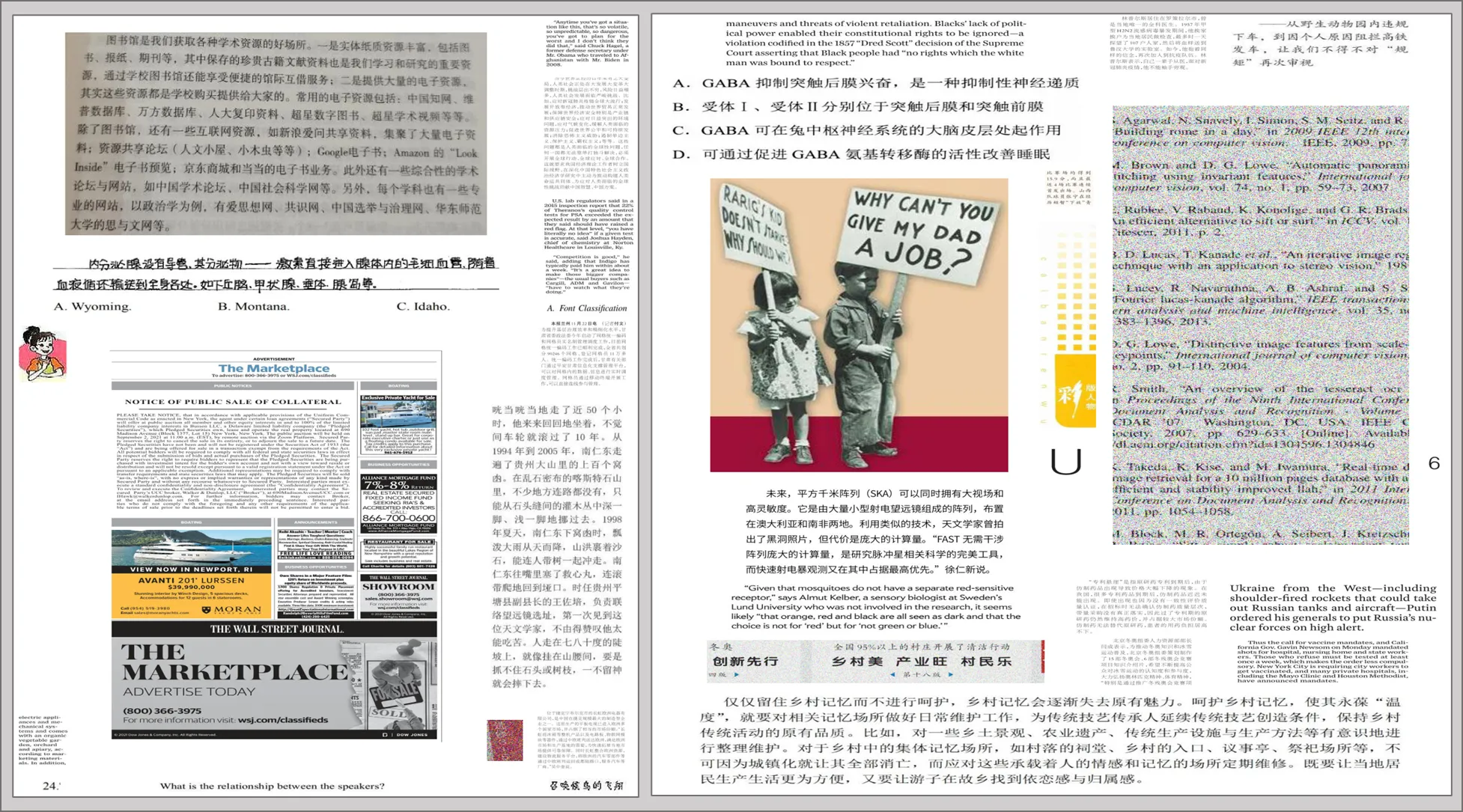
}Examples of synthetic document data.
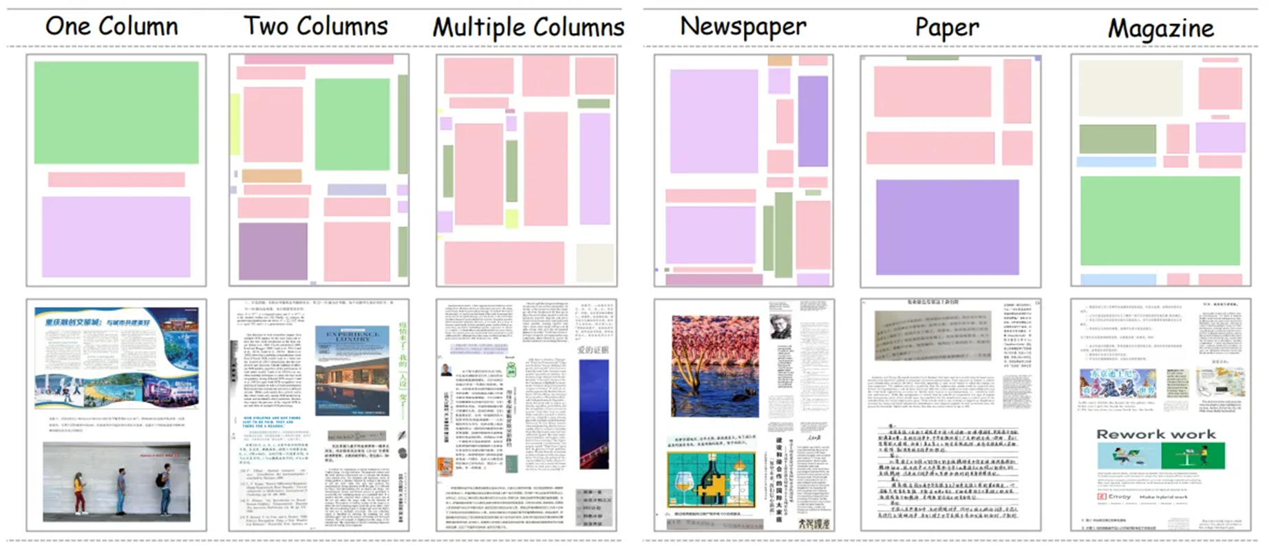
합성 문서는 포괄적인 layout 다양성 ( 다중 layout 포맷 ) 과 element 다양성 ( 다양한 요소들 통합 ) 을 보여준다. 위의 과정을 통해서 element 들은 최적의 위치에 지속적으로 채워져서 위와 같이 잘 정리되고 시각적으로 매력적인 문서 이미지를 생성한다.
생성된 문서는 높은 수준의 다양성을 나타내므로 다양한 실제 문서 유형에 효과적으로 적응하기 위해 pre-trained 모델로 가능하게 한다. 한편 정량적 분석을 통해서 생성된 문서가 alignment (정렬) 및 density (밀도) 와 같은 인간 설계 원칙을 충실하게 준수한다는 것을 보여준다.
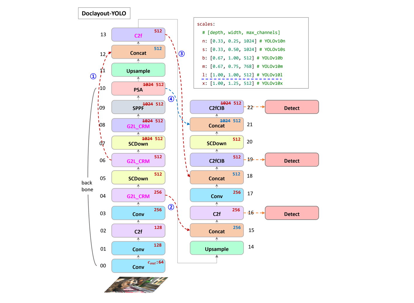
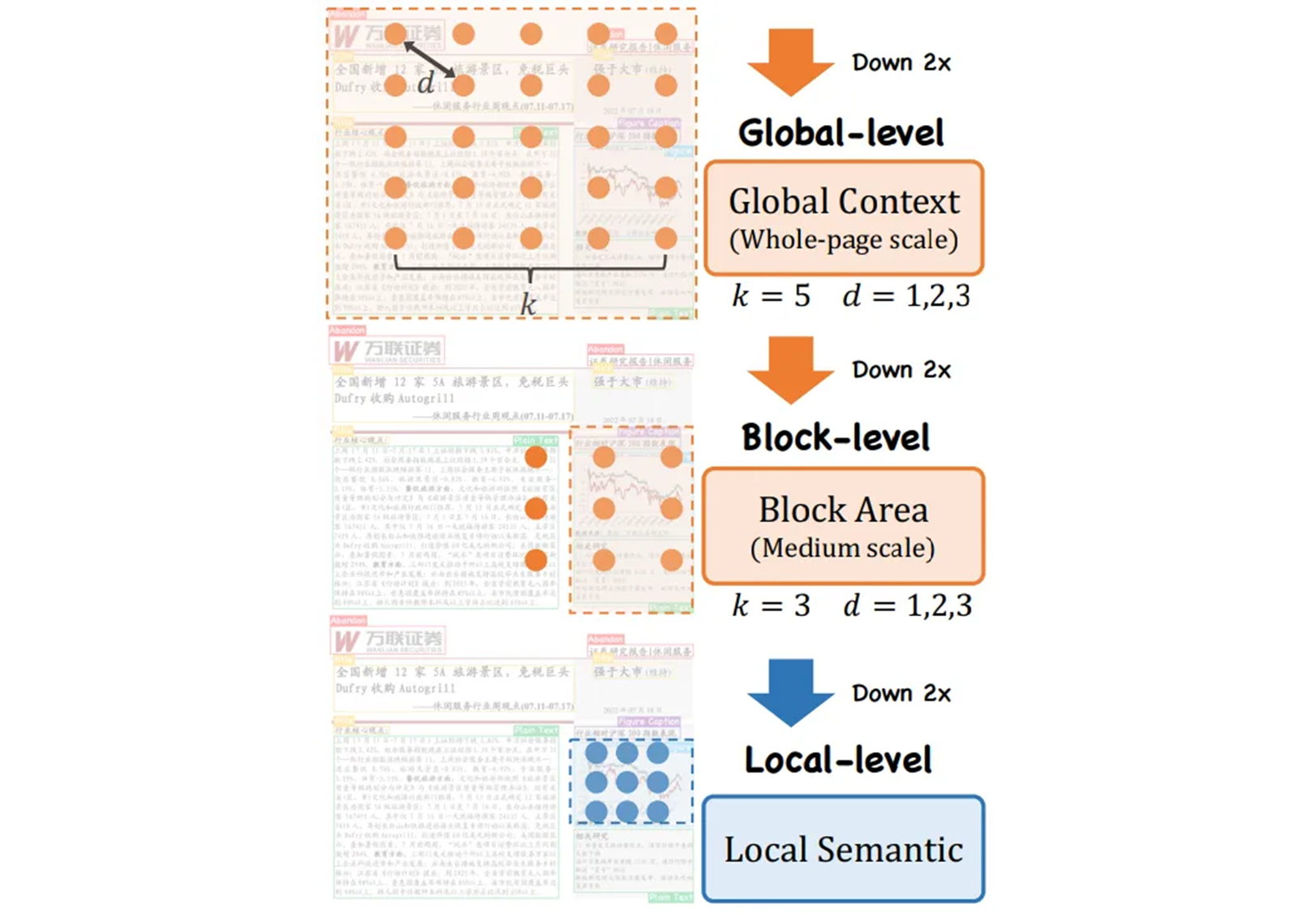
G2L_CRM (Global-to-Local model architecture)
자연스로운 이미지와는 달리, 문서 이미지의 다양한 요소는 한 줄 제목, 전체 페이지 표와 같이 크게 다를 수 있다. 이러한 규모 변화를 처리하기 위해서 CRM (Controllable Receptive Module) 와 GL (Global-to-Local Design) 인 두 가지 주요 구성 요소들로 구성된 CL-CRM 으로 불리는 계층적인 architecture 를 도입한다.
CRM 은 다양한 규모와 세분화된 기능을 유연하게 추출하고 통합하는 반면, GL 아키텍쳐는 global context (전체 페이지 규모) 에서 하위 블록 영역 ( medium-scale ), 최종적으로 로컬 의미 정보에 이르는 계층적 인식 프로세스를 제공한다.
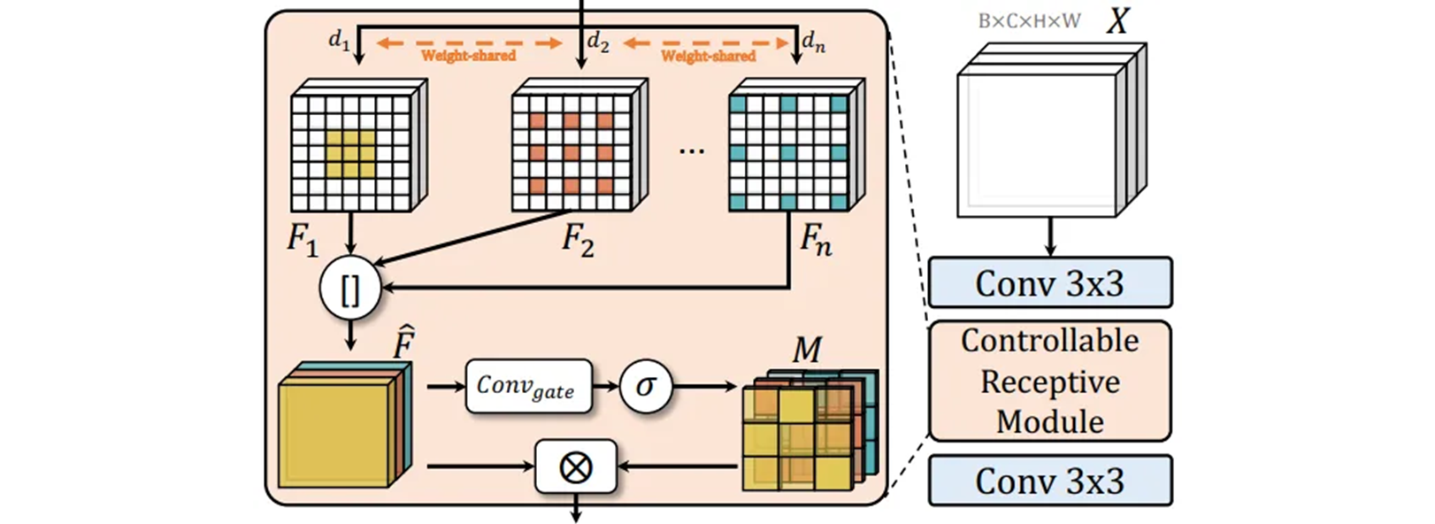
다양한 규모와 세분화의 기능을 추출하고 융합하는 Controllable Receptive Module (CRM).
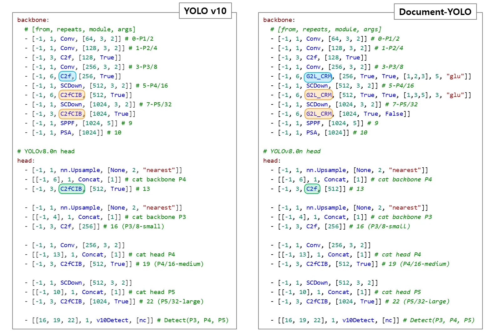
C2fCIB: Faster Implementation of CSP Bottleneck with 2 convolutions.
C2f: Faster Implementation of CSP Bottleneck with 2 convolutions.
G2L_CRM: Faster Implementation of CSP Bottleneck with 2 convolutions.
    # shortcut : True, dilated : True, block_k : 5, fuse : glu
  - [-1, 6, G2L_CRM, [256, True, True, [1,2,3], 5, "glu"]]
    # shortcut : True, dilated : True, block_k : 3, fuse : glu
  - [-1, 6, G2L_CRM, [512, True, True, [1,3,5], 3, "glu"]]
    # shortcut : True, dilated : False
- [-1, 6, G2L_CRM, [1024, True, False]]C2f,C2fCIB를G2L_CRM으로 바꿔 사용했다.- head 에서 처음 block 을
C2fCIB에서C2f만 사용한 것은 흥미롭다.-
이 말은 Pointwise, Depthwise Conv 로 reduction 을 하지 않았다는 뜻.
code 를 보면 알 수 있는데
-
기존
C2f에는self.m에Bottleneck만 들어가 있는 반면self.m = nn.ModuleList( Bottleneck( self.c, self.c, shortcut, g, k=((3, 3), (3, 3)), e=1.0 ) for _ in range(n) ) -
G2L_CRM에서 Local-level 은 Bottleneck 대신 CIB 가 들어가 있다.```python self.m = nn.ModuleList(CIB( self.c, self.c, shortcut, e=1.0) for _ in range(n) ) ```따라서
CIB가 들어가 있어서, 마지막에C2f만 넣은 듯 하다.
-
- 논문에서는
dilation이 global, block level 모두[1, 2, 3]인데 code 에서 block level 은[1, 3, 5]로 나와 있다.
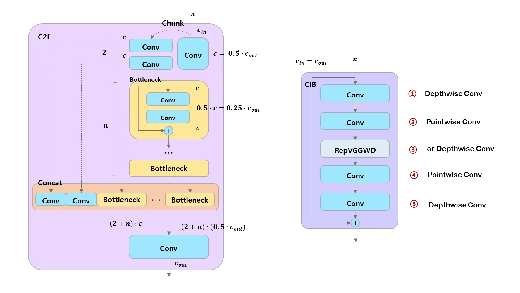
C2f와의 코드 차이는use_dilated이True면DilatedBottleneck으로self.m이 구성되고use_dilated이False이면CIB로self.m이 구성된다.
CRM (Controllable Receptive Module)
자세하게 설명하자면, 각 레이어의 특징 에 대해 커널 크기 를 갖는 weight-shared convolution 레이어 를 사용하여 특징 추출부터 시작한다.
def __init__(self, c1, c2, k=1, s=1, p=None, g=1, d=1, act=True):
    """Initialize Conv layer with given arguments including activation."""
    super().__init__()
    self.conv = nn.Conv2d(c1, c2, k, s, autopad(k, p, d), groups=g, dilation=d, bias=False)
    self.bn = nn.BatchNorm2d(c2)
    self.act = self.default_act if act is True else act if isinstance(act, nn.Module) else nn.Identity()
다양한 세분성의 특징을 잡기 위해 다양한 dilation rates 세트를 사용한다. 이 접근 방식을 사용하면 같이 표시되는 다양한 세분화의 기능 집합을 얻을 수 있다.
def dilated_conv(self, x, dilation):
    act = self.dcv.act
    bn = self.dcv.bn
    weight = self.dcv.conv.weight
    padding = dilation * (self.k//2)
    return act(bn(F.conv2d(x, weight, stride=1, padding=padding, dilation=dilation)))
다양한 세분화된 특징 추출을 통해서 이러한 기능들을 통합하고 network 가 다양한 기능 구성 요소를 자율적으로 융합하는 방법을 학습할 수 있도록 한다.
커널 크기가 1 이고 그룹이 있는 lightweight convolution layer 를 사용하여 과 사이의 값을 갖는 마스크 을 추출한다.
dx = torch.cat(dx, dim=1)
G = torch.sigmoid(self.conv_gating(dx))
dx = dx * G  # Element-wise multiplication
dx = self.conv1x1(dx)self.conv_gating = Conv(c*len(self.dilation), c*len(self.dilation), k=1, s=1, g=c*len(self.dilation))
# Conv
def forward(self, x):
"""Apply convolution, batch normalization and activation to input tensor."""
return self.act(self.bn(self.conv(x)))은 다양한 feature 들을 위한 중요한 weight 으로 생각할 수 있다. 마지막으로 은 세분화 된 특징들이 융합된 에 적용되고, 이어서 lightweight output projector 이 적용된다. 추가적으로 초기 feature 를 통합 feature 와 병합하는데 shortcut connection 이 사용된다.
return x + dx if self.add else dx은 다양한 세분화의 feature 들을 추출하고 강화하기 위해서 전통적인 CSP bottleneck 에 연결한다. 의 기능은 추출된 기능의 세부성과 규모를 제어하는 두 개의 parameter 에 의해 제어된다.
GL (Global-to-Local design)
- Dilation 개념을 보자.
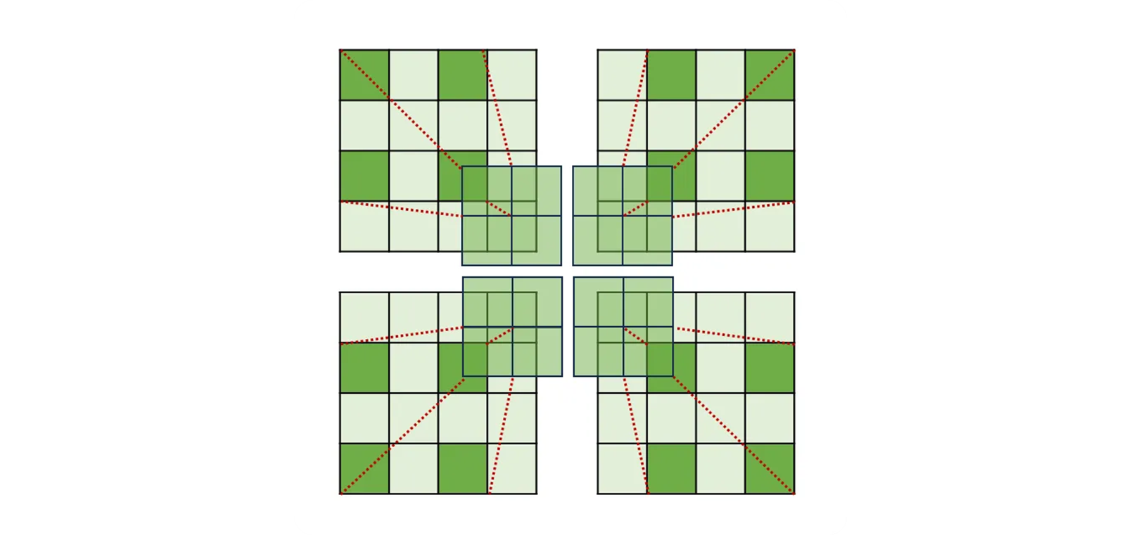
- 2D Conv 에서 kernel 2, dilation rate 2 가 되고,
- view 는 중간에 비어 있지만 kernel 3 의 시야를 갖게 된다.
Global-level
풍부한 텍스처의 detail 들이 포함된 얕은 stage 의 경우에는 확대된 kernel 사이즈 , dilation rate 를 CRM 에서 사용한다. 큰 kernel 은 더 많은 텍스쳐 detail 들을 잡아내고, 전체 page 요소에 대한 local 패턴을 보존하는데에 도움이 된다.

[-1, 6, G2L_CRM, [256, True, True, [1,2,3], 5, "glu"]]Block-level
feature map 이 downsample 되고 텍스처 feature 가 감소되는 중간 단계의 경우에는 더 작은 커널 을 CRM 에서 사용한다. 이 경우 확장된 dilation rate 은 문서 하위 블록과 같은 중간 규모 요소들의 인식을 위해 충분하다.

[-1, 6, G2L_CRM, [512, True, True, [1,3,5], 3, "glu"]]논문에서는 dilation 이 [1, 2, 3] 인 반면 코드에서는 [1, 3, 5] 로 더 넓게 펴서 시야를 넓혔다.
Local-level
의미 정보가 우세한 깊은 stage 의 경우에는 로컬 의미 정보에 초점을 맞춘 경량화 모듈 역할을 하는 기본 bottleneck 을 사용한다.

[-1, 6, G2L_CRM, [1024, True, False]]False 로 하는 대신 CIB 를 사용하여 13 layer 에서 기존 C2fCIB 대신 C2f 로 시작한다.
Model Architecture Overview