overview
advantages of opencv-based programs
-
빠른 속도
- 비교적 간단한 모델을 사용하여 빠르게 객체 탐지 가능
- 이 말은 task 가 쉬워야 한다. 일반화 모델에는 적절하지 못할 가능성이 높다.
-
낮은 자원 사용
- 딥러닝 모델에 비해 메모리와 연산 자원이 덜 사용
- 현재 gpu 의 성능이 너무 많이 올라왔고, computation cost 가 인력 비용 대비 적게 들어간다.
-
사용하기 쉬움
- OpenCV document 와 tutorial 이 너무 잘나와있다. + GPT 를 합하면 너무 편하게 쓴다.
-
전처리 기능 풍부
- 이미지 preprocessing 및 기타 컴퓨터 비전 작업에 유용한 기능들이 많다.
- 이번 post 도 opencv 를 사용할 것이며, 한 단계씩 넘어가볼 예정이다.
drawbacks of opencv-based programs
- 정확도
- 딥러닝 기반 모델에 비해 정확도가 낮을 수 있다.
- 많이 차이난다. 특히 나 같은 OpenCV 를 세밀하게 다뤄보지 못한 사람 한테는..
- 제한된 범용성
- 특정 객체나 환경에서 잘 동작하지만, 다양한 객체에 대한 일반화가 어려울 수 있다.
- 이게 진짜 치명적인 단점이다. 정말 필요한 객체만을 볼 때는 쉽게 쓸수 있다.
- 현재 대부분의 task 들이 딥러닝 계열로 쉬워져서, 일반화를 고려해야 한다.
another example
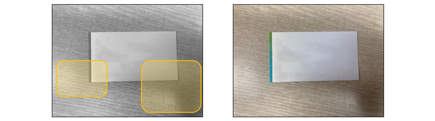
아주 살짝 그림자가 지고, 아주 살짝 빛 반사가 된 약간 어려운 task 를 가져와 봤다.
pixel distribution
import cv2
import seaborn as sns

src = cv2.imread(IMG_PATH)
src_gray = cv2.cvtColor(src, cv2.COLOR_BGR2GRAY)

sns.histplot(src_gray.reshape(-1,))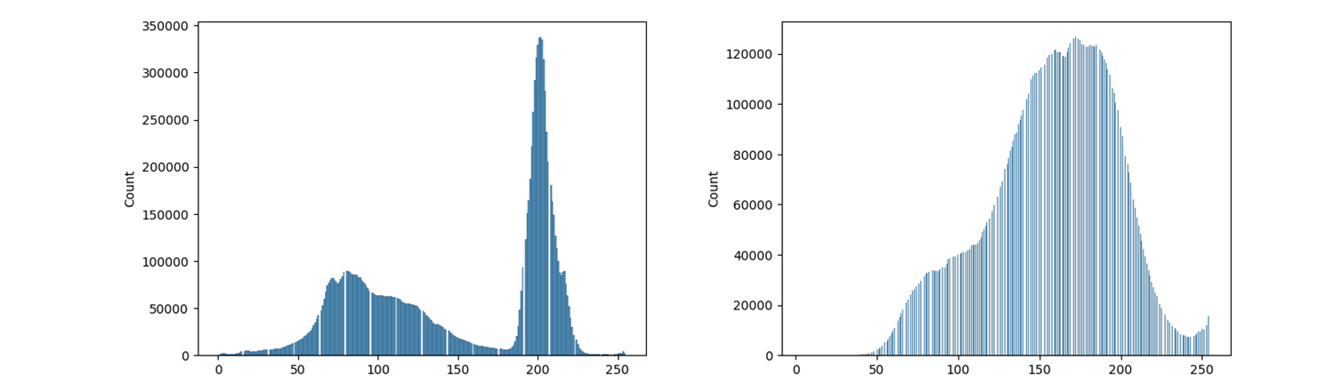
확실히 이전 post 보다 훨씬 어려워진 분포가 된다.
threshold
src = cv2.imread(IMG_PATH)
src_gray = cv2.cvtColor(src, cv2.COLOR_BGR2GRAY)

th, src_bin = cv2.threshold(src_gray, 0, 255, cv2.THRESH_BINARY | cv2.THRESH_OTSU)
print("Auto threshold:", th)

fig = plt.figure(figsize=(10,10))

ax1 = fig.add_subplot(1, 2, 1)
ax1.imshow(cv2.cvtColor(src_gray, cv2.COLOR_BGR2RGB))
ax1.set_title("1st pic", fontsize=10)

ax2 = fig.add_subplot(1, 2, 2)
ax2.imshow(cv2.cvtColor(src_bin, cv2.COLOR_BGR2RGB))
ax2.set_title("2th pic", fontsize=10)
Auto threshold: 150.0 으음.. 150 정말 맞나..
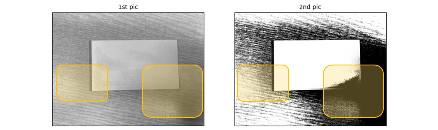
다음 번 예시는 아예 빛 반사와 흰 배경으로 가져와야지.. 오른쪽만 좀 침범 해서 현재 코드로는 탐지하기 어려울 듯, 앞단에 좀 더 preprocessing 이 들어가고 minAreaRect 을 넣어 그려볼 예정.
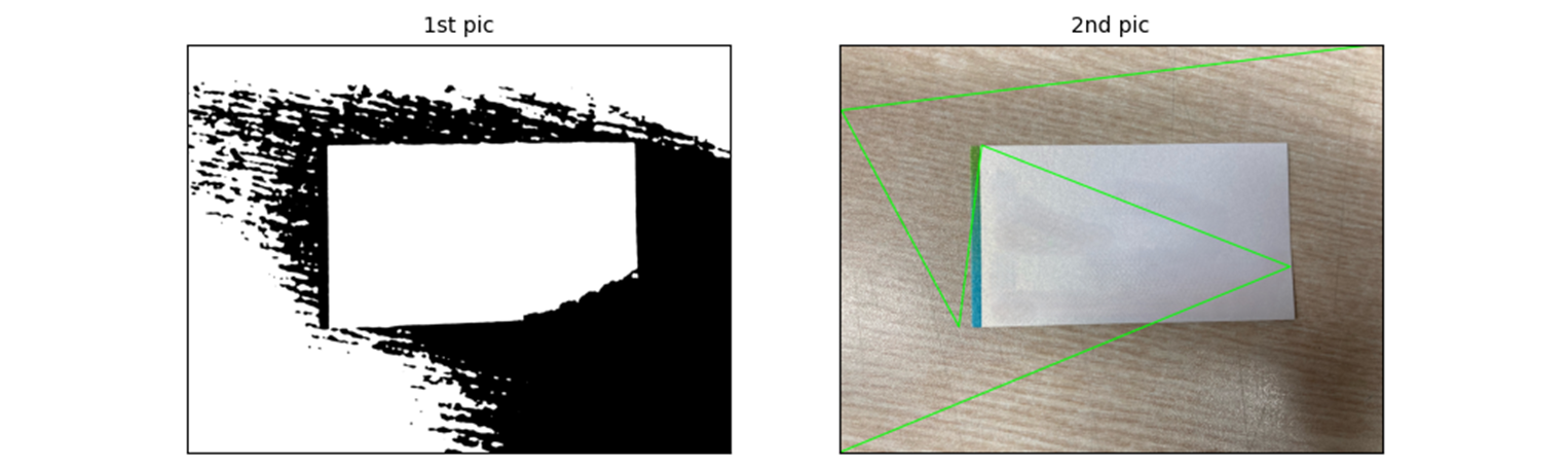
find contour
# Contour detection
contours, _ = cv2.findContours(src_bin, cv2.RETR_EXTERNAL, cv2.CHAIN_APPROX_NONE)

for contour in contours:

    # Ignore small object
    if cv2.contourArea(contour) < 20000:
        continue

    # Contour approximation
    epsilon = 0.02 * cv2.arcLength(contour, True)
    approx = cv2.approxPolyDP(contour, epsilon, True)

    # If approximated as a rectangle, draw the contour.
    if len(approx) == 4:
        cv2.polylines(src, [approx],
                isClosed=True,
                color=(0, 255, 0),
                thickness=30,
                lineType=cv2.LINE_AA
)plt.imshow(cv2.cvtColor(src, cv2.COLOR_BGR2RGB))
plt.xticks([])
plt.yticks([])
plt.show()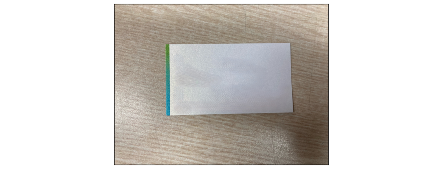
잡힐 턱이 있나..
if cv2.contourArea(contour) < 2000:임계치를 줄이면,

이런 식으로 나온다.
preprocessing update and upgrade
src_gray = cv2.medianBlur(src_gray, 21)
src_gray = cv2.bilateralFilter(src_gray, -1, 50, 10)-
GaussianBlur를 일반적으로 사용하긴 하지만, 세밀하게 작업하는 목적이 아니라서.. -
bilateralFilter(src, d, sigmaColor, sigmaSpace, dst=None, borderType=None)- 가장자리 보존 필터로 이미지를 blur 처리하고 가장자리 정보를 유지.
d: 필터링에 사용할 각 픽셀 이웃의 지름.d가 음수이면sigmaSpace값에 의해 자동 계산.sigmaColor: 색 공간에서 필터의 sigma.- 이 값이 클 수록 더 넓은 색 범위에서 pixel 이 혼합.
- 색상의 차이가 큰 pixel 도 혼합될 수 있다.
sgmaSpace: 좌표 공간에서 filter 의 sigma.- 이 값이 클 수록 더 넓은 pixel 이웃이 혼합된다.
- 좌표 공간에서 거리가 멀어도 필터링에 포함될 수 있다.
를 추가하고, contourArea 를 20000 으로 다시 원복하고,
if cv2.contourArea(contour) < 20000:일단 무엇을 그리는지 확인하기 위해서
if len(approx) == 4:의 조건을 빼고 그려보면,
gamma up
그림자의 문제가 되면 gamma 를 추가 하여 좀더 밝게 해보면
gamma = 1.1
src_gray = src_gray.astype(np.float32)
src_gray = ((src_gray / 255) ** (1 / gamma)) * 255
src_gray = src_gray.astype(np.uint8)
minAreaRect
이렇게 선을 approximation 하지 말고, minAreaRect 를 사용하여 사각을 그려보고 그 box 들을 활용하여 그려보는 것이 더 알맞을 것으로 판단.
- minAreaRect
주어진 2D point set 에 대해서 최소 면적의 회전된 사각형rotated bounding box을 계산한다.
# Contour detection
contours, _ = cv2.findContours(src_bin, cv2.RETR_EXTERNAL, cv2.CHAIN_APPROX_NONE)

for contour in contours:
    rect = cv2.minAreaRect(contour)
    box = cv2.boxPoints(rect)
    box = np.intp(box)

    # Ignore small object
    if cv2.contourArea(box) < 20000:
        continue

    cv2.drawContours(src, [box], 0, (0, 255, 0), 2)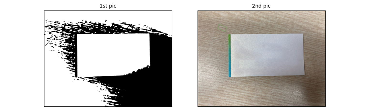
아무것도 그려지지 않는다. 1st pic 에서 edge 만 걸러보자.
canny edge detection
canny 알고리즘
- 이미지에서 edge 를 추출하는 데 사용되는 강력한 알고리즘이다.
min_val = 5
max_val = 50
edge_canny = cv2.Canny(src_gray, min_val, max_val)
를 이용 하면
fig = plt.figure(figsize=(10,10))

ax1 = fig.add_subplot(1, 3, 1)
ax1.imshow(cv2.cvtColor(edge_canny, cv2.COLOR_BGR2RGB))
ax1.set_title("1st pic", fontsize=10)

ax2 = fig.add_subplot(1, 3, 2)
edge_canny = cv2.bitwise_not(edge_canny)
ax2.imshow(cv2.cvtColor(edge_canny, cv2.COLOR_BGR2RGB))
ax2.set_title("2nd pic", fontsize=10)


ax2 = fig.add_subplot(1, 3, 3)
ax2.imshow(cv2.cvtColor(src, cv2.COLOR_BGR2RGB))
ax2.set_title("3th pic", fontsize=10)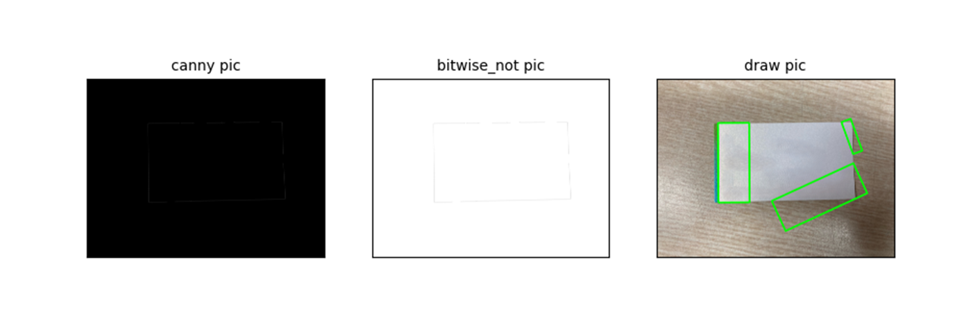
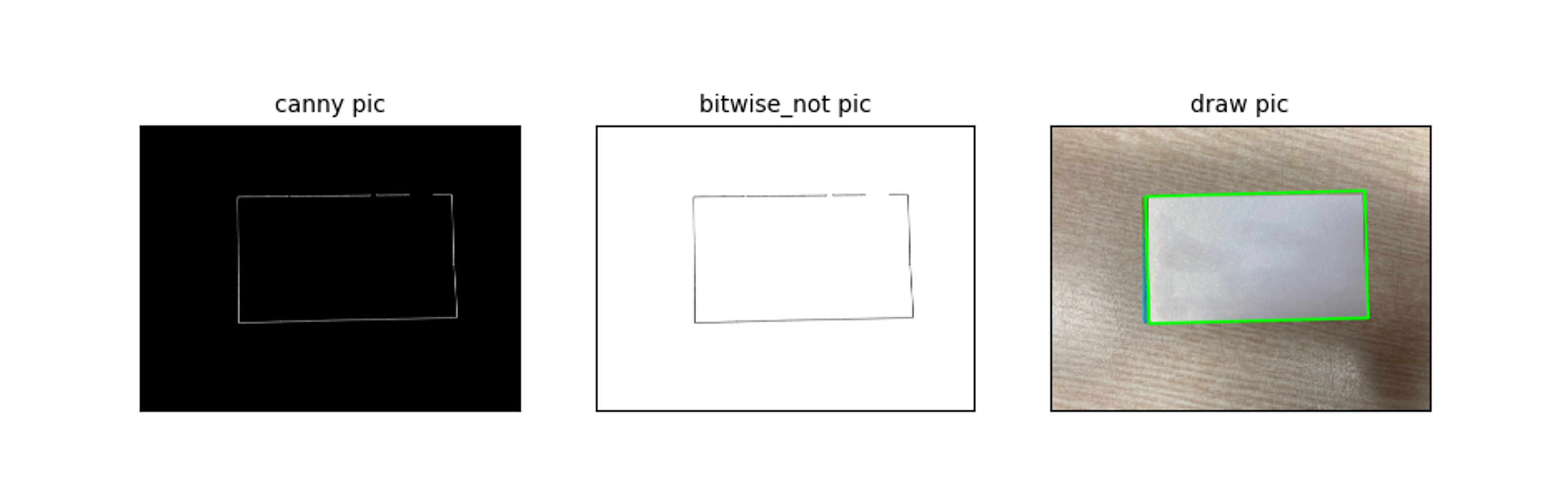
edge detection 에서 edge 가 너무 옅게 나와서 dilate 를 사용.
kernel = np.ones((3, 3), np.uint8)
edge_canny = cv2.dilate(edge_canny, kernel, iterations=3)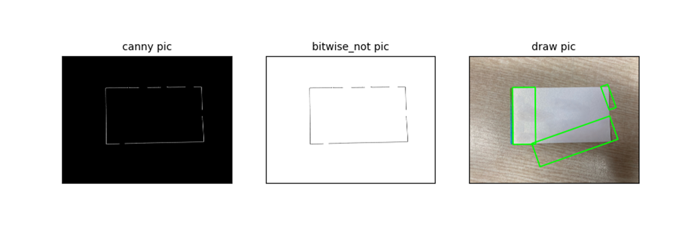
gamma down
중간에 끊어짐이 있으니 gamma 를 다시 내려서 볼까..
gamma = 1
오 ... 그렇네..
result

자세히 보면, 정확한 fit 은 되지 않았다. 일단 넘어가고, 좀 더 어려운 task 가져오자.
이것이 일반화 시키려는 방법인데, 앞서 언급했지만, 제한된 범용성 이것이 정말 어렵다.
Just with 'openCV' alone....