1.PCA Concept
1.1. Point
-
PCA 는 차원이 정해져 있지 않다. 데이터를 보고 연구자가 직접 정해야 한다.
- 그 판단이 한 가지만 있는 것이 아니고, 여러 가지 방법들이 있다.
- eigenvalue, eigenvector 를 통해 변환을 해서 주성분을 구하게 된다.
-
차원의 축소가 목적, 이렇게 나온 주성분 (principle component) 들이 서로 상관되어 있지 않다. (독립적)
- 첫 번째 주성분이 구해지면, 다음 주성분은 상관되어 있지 않은 새로운 변수 주성분으로 만든다.
- 가 상관관계가 높은 (비슷한) 변수면, 둘 다 필요가 없다.
- 주성분 끼리 상관이 되어 있으면, 설명을 겹쳐서 하는 일이 발생, 독립적 이어야 남은 부분을 설명.
-
Example 에서는 주성분이 1개 이지만, 2개, 3개, ... 개 로 구할 수 있다.
- 각 변수들의 선형 결합으로 이루어진 사실은 평균 구하는 것과 같다.
- 첫 번째 주성분의 데이터에 최대한 설명할 수 있도록, 힘을 실어 주는 것.
- 주성분의 weight 은 와 같이 weight 을 준 것.
- weight 은 낮을 수록 설명력이 낮아진다고 볼수 있다.
- 주성분을 구한 후, 어느 시점에 끊어서 개만 이용하자고 정하는 것.
- PCA 점수 (loading) 은 동일한 제약조건을 가지는 모든 가능한 선형 결합 중 가장 변이가 크다.
- 변이가 크다 : 데이터의 분산을 많이 설명한다는 뜻이다.
- 주성분이 상관이 많이 되어 있어야 이들을 잘 설명하는 것이 된다.
- PCA 를 통해 얻은 주성분계수의 상대적 크기를 이용한다.
1.2. Example
1.2.1. Table
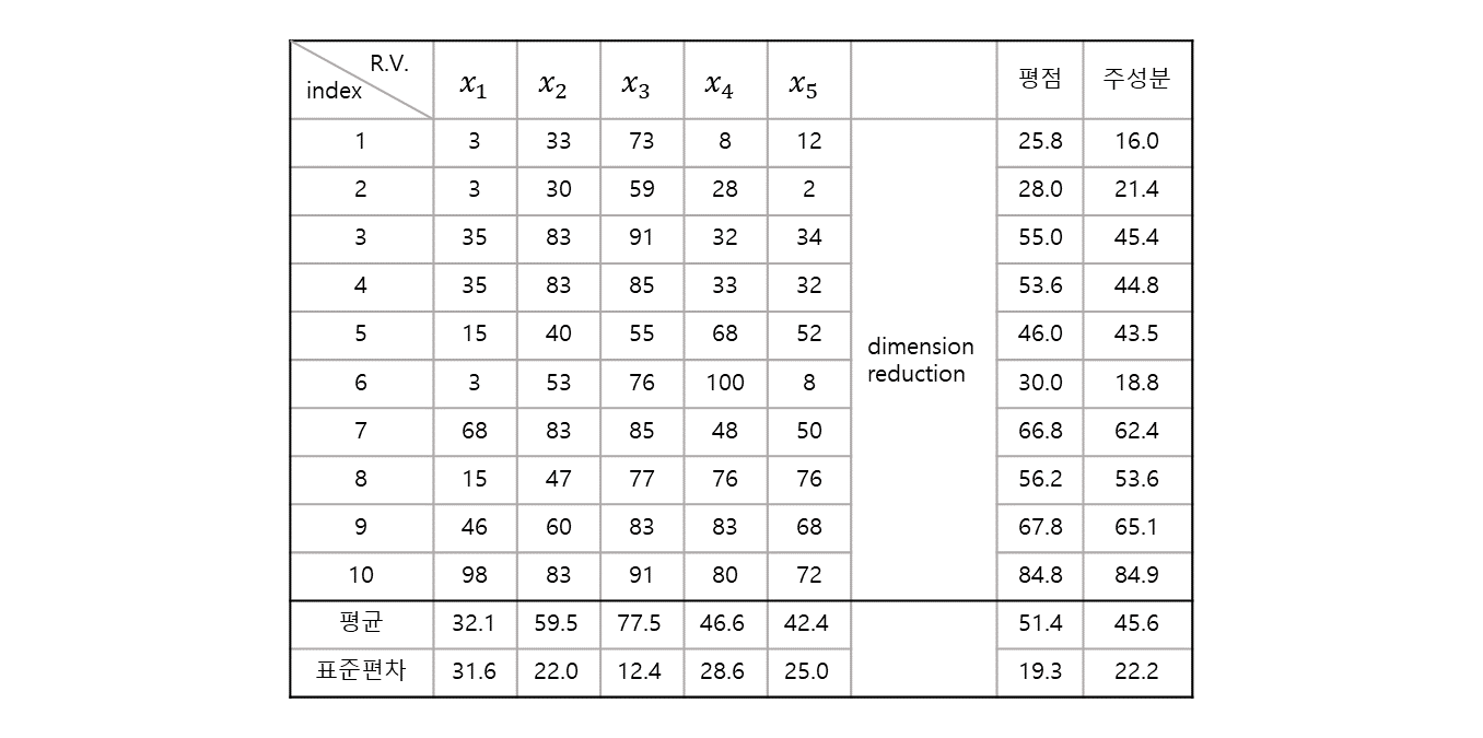
변수 : (5개)
샘플 : 10개
-
5 차원의 데이터라고 볼 수 있다.
- 차원 축소를 하는데, 가장 많이 사용 하는 것은 "평균 (mean)" 을 사용하면 된다.
- 5 개 값의 평균을 내보면, "평점" 이라는 변수가 생기고, 각 변수에 대한 정보들이 어느 정도 반영 된다.
-
차원 축소의 관점에서 보자면 평균은 5 개의 과목을 하나의 점수로 구한 것 자체가 차원의 축소가 일어난 것.
각 성분() 별 weight 을 을 준 것.
-
행렬의 Variance, Covariance 등을 이용하여 어떻게 하면 차원을 축소 하면서 정보의 손실양을 minimize 할 수 있는지를 만들어 보는 방법 대표적으로 PCA 가 그러한 방법.
1.2.2. 3D-image
source : https://www.ty-penguin.org.uk/~auj/old_aber_pages/talks/depttalk96/pca.active.html
처음에는 자료의 점들의 구조를 파악하기 힘드나, 적절한 회전을 하면 숨겨진 구조가 나온다. 자료 주위를 돌면서 가장 적절한 관찰 방향을 찾는 것과 같은 의미.
데이터의 손실이 있으나, 3차원의 data 모습이 2차원으로도 뚜렷하게 보이게 된다.
- 3차원 데이터를 2차원으로 줄였으니, 차원 축소가 일어난 것이다.
- 설명을 위해서 3차원 이지만, 실제 데이터는 수십개의 차원을 줄여서 줄인 차원으로 분석한다.
- 어떤 방향에서 봐야 적절할까, 가장 데이터에 변동이 잘 보일까를 찾는 것이 PCA.
예를 들어 의 설명력을 위해서는 100 차원을 써야 하는데, 의 설명력을 위해 10차원만 써도 되면
자료의 손실 를 감안 하더라도 후자를 사용하는 것이 noise 제거와 데이터 효율성을 위해 나은 선택이 된다.
대부분의 분산 (variance) 이 처음 몇 개의 차원에 표현 되도록 회전을 시킨다.
1.2.3. 3D-space
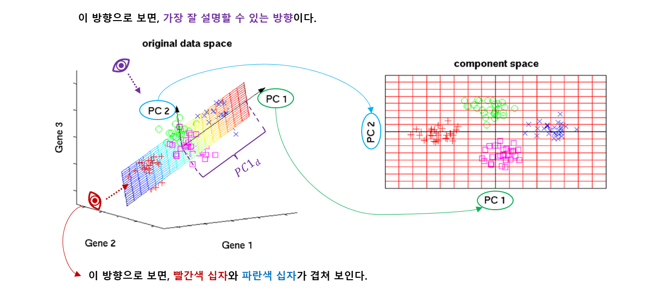
: 가장 데이터의 변동을 잘 잡아주는 주성분.
: 첫 번째 eigenvector 의 eigenvalue .
- 두 주성분은 기하학적으로는 직교, 통계적으로는 독립 (서로 상관되어 있지 않다).
- 각각 의 선형 결합으로 만들어 진다.
- 각각의 방향이 eigenvector 가 하는 역할이 된다.
- 최대한 자료가 잘 퍼져 있는 분산을 최대화 하면서 차원을 축소 시킨다.
- eigendecomposition of a matrix 참고.
- covariance matrix 는 symmetric matrix.
- https://en.wikipedia.org/wiki/Eigendecomposition_of_a_matrix#Decomposition_for_special_matrices
1.2.4. Explanation
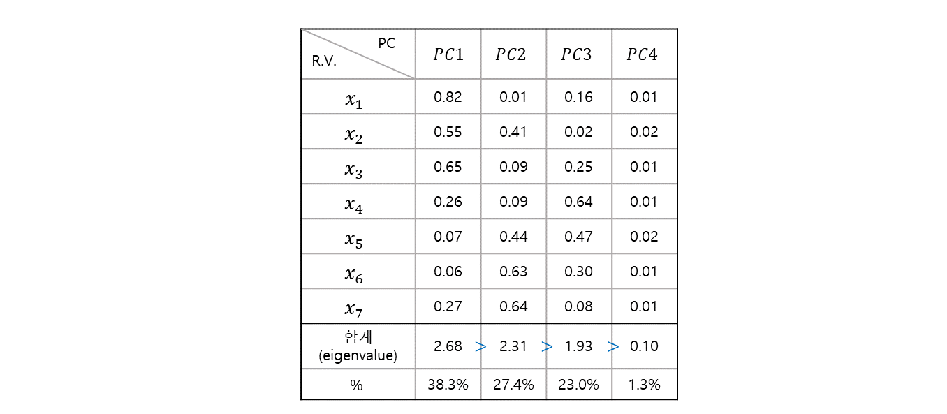
주성분 이 어떻게 들의 선형 결합으로 이루어져 있는지 보여주고 있다.
- 이 때, 총 data 변동의 첫 번째 주성분이 를 설명 한다.
- 평균을 생각해보면, 평균 방법은 변수 하나가 를 설명 한다.
- eigenvalue 로 sorting 하므로, 설명력은 이 제일 크고, 나머지는 그보다 낮은 설명력을 갖는다.
- 에서 잘라주고 나머지 4 개의 주성분은 버린다.
- 약 설명력을 하면서, 약 의 데이터 손실은 있으나, 7차원에서 3차원으로 줄였다.
2. Data analysis
2.1 preprocessing
- (가격), (성능), (편리성), (디자인), (색상)
> Satis <- read.table("satis.txt", header=T)
> Satis
   subject gender age x1 x2 x3 x4 x5
1        1      F  10  1  2  4  1  1
2        2      F  10  1  2  3  2  1
3        3      F  20  2  5  5  2  2
4        4      F  20  2  5  5  2  2
5        5      F  30  1  2  3  4  3
6        6      M  30  1  3  4  1  1
7        7      M  40  4  5  5  3  3
8        8      M  40  1  3  4  4  4
9        9      M  50  3  3  5  5  4
10 10 M 50 5 5 5 4 4- subject 삭제, variable name 설정
> Satis <- Satis[,-1]
> colnames(Satis) <- c("Gender", "Age", "Price", "Function", "Easy", "Design", "Color")
> Satis
   Gender Age Price Function Easy Design Color
1       F  10     1        2    4      1     1
2       F  10     1        2    3      2     1
3       F  20     2        5    5      2     2
4       F  20     2        5    5      2     2
5       F  30     1        2    3      4     3
6       M  30     1        3    4      1     1
7       M  40     4        5    5      3     3
8       M  40     1        3    4      4     4
9       M  50     3        3    5      5     4
10 M 50 5 5 5 4 4- summary 확인. Price, Function, Easy, Design, Color 은 5점 척도.
> summary(Satis[,3:7])
     Price         Function         Easy         Design        Color
 Min.   :1.00   Min.   :2.00   Min.   :3.0   Min.   :1.0   Min.   :1.00
 1st Qu.:1.00   1st Qu.:2.25   1st Qu.:4.0   1st Qu.:2.0   1st Qu.:1.25
 Median :1.50   Median :3.00   Median :4.5   Median :2.5   Median :2.50
 Mean   :2.10   Mean   :3.50   Mean   :4.3   Mean   :2.8   Mean   :2.50
 3rd Qu.:2.75   3rd Qu.:5.00   3rd Qu.:5.0   3rd Qu.:4.0   3rd Qu.:3.75
 Max.   :5.00   Max.   :5.00   Max.   :5.0   Max.   :5.0   Max.   :4.00
2.2 Check statistics.
- 기초 통계량 확인
- 1 : row 마다 기초 통계량 확인.
- 2 : column 마다 기초 통계량 확인.
# standard deviation
> apply(Satis[,3:7], 2, sd)
    Price  Function      Easy    Design     Color
1.4491377 1.3540064 0.8232726 1.3984118 1.2692955
# sum
> apply(Satis[,3:7], 2, sum)
Price Function Easy Design Color
21 35 43 28 25 - 피어슨 상관 계수 (Pearson correlation coefficient) 행렬
- 단위와 무관하게 scaling 을 했기 때문에 대각 원소는 항상 1이 된다.
- 비대각원소는 -1 ~ 1 사이의 값을 가지게 된다.
> cor(Satis[,3:7])
             Price   Function      Easy     Design     Color
Price    1.0000000 0.70784332 0.7171251 0.44960032 0.5738636
Function 0.7078433 1.00000000 0.8472509 0.05868157 0.2909287
Easy     0.7171251 0.84725089 1.0000000 0.15441829 0.3721509
Design   0.4496003 0.05868157 0.1544183 1.00000000 0.9389683
Color 0.5738636 0.29092868 0.3721509 0.93896829 1.0000000- 공분산(covariance) 행렬
- scaling 전 이라서 분산이 1 넘어가는 것을 확인할 수 있다.
> cov(Satis[,3:7])
             Price  Function      Easy    Design     Color
Price    2.1000000 1.3888889 0.8555556 0.9111111 1.0555556
Function 1.3888889 1.8333333 0.9444444 0.1111111 0.5000000
Easy     0.8555556 0.9444444 0.6777778 0.1777778 0.3888889
Design   0.9111111 0.1111111 0.1777778 1.9555556 1.6666667
Color 1.0555556 0.5000000 0.3888889 1.6666667 1.6111111- eigenvalue 와 eigenvector 를 구해주는 함수.
- eigenvectors 는 -th 주성분이 어떤 방향으로 가는지 나타낸다.
- eigenvalues 는 내림차순으로 sorting 됨을 알 수 있다.
- eigenvalues 는 eigenvectors 의 크기.
> eigen(cov(Satis[,3:7]))
eigen() decomposition
$values
[1] 5.08214264 2.45818249 0.44411043 0.14197348 0.05136875

$vectors
           [,1]       [,2]        [,3]        [,4]       [,5]
[1,] -0.5737259 -0.2558755  0.77345688 -0.04239327  0.0730312
[2,] -0.4101979 -0.5814345 -0.50999927 -0.46583216 -0.1287354
[3,] -0.2600413 -0.2859829 -0.22302049  0.87797754 -0.1732328
[4,] -0.4523733  0.6017424 -0.08005497 -0.08610099 -0.6476437
[5,] -0.4799096  0.3906169 -0.29243507  0.05427026  0.7270775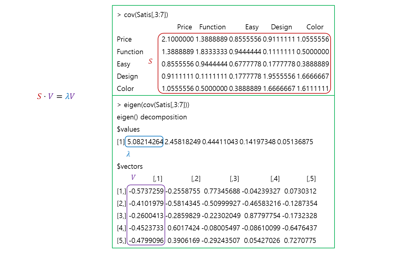
S = cov(Satis[,3:7])

# eigenvalue
lambda = eigen(cov(Satis[,3:7]))$values

# eigenvector
V = eigen(cov(Satis[,3:7]))$vectors> S %*% matrix(V[,1])
[,1]
Price -2.915757
Function -2.084684
Easy -1.321567
Design -2.299026
Color -2.438969> lambda[1] * matrix(V[,1])
[,1]
[1,] -2.915757
[2,] -2.084684
[3,] -1.321567
[4,] -2.299026
[5,] -2.438969=
2.3 Principle Component (PC)
- centering 을 한다는 것은 평균을 0으로 맞춘다는 의미.
- scaling 을 한다는 것은 분산으로 나눠주는 것이므로
- scaling 을 하면 Pearson correlation coefficient matrix 로 주성분 분석
- scaling 을 안하면 covariance matrix 로 주성분 분석
일반적으로 scaling 을 하지만, 만족도 조사는 1, 2, 3, 4, 5 밖에 없으므로, 굳이 scaling 을 안해도 된다.
변수들의 단위가 같다면, scaling 의 차이가 없다. 단위가 다르다면 (키, 몸무게 등..) scaling 을 해야한다.
> pca_model = prcomp(Satis[,3:7], center=TRUE, scale=FALSE)
> pca_model

# eigenvalues 와 관련 있다.
Standard deviations (1, .., p=5):
[1] 2.2543608 1.5678592 0.6664161 0.3767937 0.2266467

# eigenvector 와 관련 있다.
Rotation (n x k) = (5 x 5):
               PC1        PC2         PC3         PC4        PC5
Price    0.5737259  0.2558755  0.77345688  0.04239327  0.0730312
Function 0.4101979  0.5814345 -0.50999927  0.46583216 -0.1287354
Easy     0.2600413  0.2859829 -0.22302049 -0.87797754 -0.1732328
Design   0.4523733 -0.6017424 -0.08005497  0.08610099 -0.6476437
Color    0.4799096 -0.3906169 -0.29243507 -0.05427026  0.7270775
>
2.3.1 eigenvalue, eigenvector.
-
eigenvalue
Standard deviations (1, .., p=5): [1] 2.2543608 1.5678592 0.6664161 0.3767937 0.2266467값 으로
> pca_model$sdev^2
[1] 5.08214264 2.45818249 0.44411043 0.14197348 0.05136875
이면
# eigenvalue
eigen(cov(Satis[,3:7]))$values
[1] 5.08214264 2.45818249 0.44411043 0.14197348 0.05136875
와 같게 나온다.
-
eigenvector
Rotation (n x k) = (5 x 5):
           PC1        PC2         PC3         PC4        PC5
Price    0.5737259  0.2558755  0.77345688  0.04239327  0.0730312
Function 0.4101979  0.5814345 -0.50999927  0.46583216 -0.1287354
Easy     0.2600413  0.2859829 -0.22302049 -0.87797754 -0.1732328
Design   0.4523733 -0.6017424 -0.08005497  0.08610099 -0.6476437
Color    0.4799096 -0.3906169 -0.29243507 -0.05427026  0.7270775
직교는 90도, 수직의 의미이고, 는 서로 직교한다.
대수적으로 보면 내적의 합이 의 의미이다.> sum(pca_model$rotation[,1] * pca_model$rotation[,2]) [1] -6.938894e-17 > sum(pca_model$rotation[,1] * pca_model$rotation[,5]) [1] -9.714451e-17 > sum(pca_model$rotation[,3] * pca_model$rotation[,5]) [1] 5.551115e-17이 정도면 0으로 봐도 무방하다. (torch 에선 -37 정도 되어야 0으로 본다.)
rotation 은, 축을 돌려서 가장 잘 표현하는, 위에서 말한 펭귄 을 생각하면 된다.
마다 eigenvector 와 비교 시 부호가 같거나 바뀌어 있음을 알 수 있다.$vectors [,1] [,2] [,3] [,4] [,5] [1,] -0.5737259 -0.2558755 0.77345688 -0.04239327 0.0730312 [2,] -0.4101979 -0.5814345 -0.50999927 -0.46583216 -0.1287354 [3,] -0.2600413 -0.2859829 -0.22302049 0.87797754 -0.1732328 [4,] -0.4523733 0.6017424 -0.08005497 -0.08610099 -0.6476437 [5,] -0.4799096 0.3906169 -0.29243507 0.05427026 0.7270775은 단위 고유 vector 이므로, 길이가 1이 된다.
> sum(pca_model$rotation[,2]^2)
[1] 1
> sum(pca_model$rotation[,4]^2)
[1] 1
2.3.2 eigen decomposition
source : https://en.wikipedia.org/wiki/Eigendecomposition_of_a_matrix#Decomposition_for_special_matrices
> pca_model$rotation PC1 PC2 PC3 PC4 PC5 Price 0.5737259 0.2558755 0.77345688 0.04239327 0.0730312 Function 0.4101979 0.5814345 -0.50999927 0.46583216 -0.1287354 Easy 0.2600413 0.2859829 -0.22302049 -0.87797754 -0.1732328 Design 0.4523733 -0.6017424 -0.08005497 0.08610099 -0.6476437 Color 0.4799096 -0.3906169 -0.29243507 -0.05427026 0.7270775> diag(pca_model$sdev^2) [,1] [,2] [,3] [,4] [,5] [1,] 5.082143 0.000000 0.0000000 0.0000000 0.00000000 [2,] 0.000000 2.458182 0.0000000 0.0000000 0.00000000 [3,] 0.000000 0.000000 0.4441104 0.0000000 0.00000000 [4,] 0.000000 0.000000 0.0000000 0.1419735 0.00000000 [5,] 0.000000 0.000000 0.0000000 0.0000000 0.05136875> t(pca_model$rotation) Price Function Easy Design Color PC1 0.57372594 0.4101979 0.2600413 0.45237328 0.47990955 PC2 0.25587549 0.5814345 0.2859829 -0.60174239 -0.39061690 PC3 0.77345688 -0.5099993 -0.2230205 -0.08005497 -0.29243507 PC4 0.04239327 0.4658322 -0.8779775 0.08610099 -0.05427026 PC5 0.07303120 -0.1287354 -0.1732328 -0.64764368 0.72707753> pca_model$rotation%*%diag(pca_model$sdev^2)%*%t(pca_model$rotation) Price Function Easy Design Color Price 2.1000000 1.3888889 0.8555556 0.9111111 1.0555556 Function 1.3888889 1.8333333 0.9444444 0.1111111 0.5000000 Easy 0.8555556 0.9444444 0.6777778 0.1777778 0.3888889 Design 0.9111111 0.1111111 0.1777778 1.9555556 1.6666667 Color 1.0555556 0.5000000 0.3888889 1.6666667 1.6111111
PCA를 활용하여 3개의 Matrix 를 구하고, 곱하여서 공분산 행렬을 구하게 된다.
- Covariance matrix
> cov(Satis[,3:7]) Price Function Easy Design Color Price 2.1000000 1.3888889 0.8555556 0.9111111 1.0555556 Function 1.3888889 1.8333333 0.9444444 0.1111111 0.5000000 Easy 0.8555556 0.9444444 0.6777778 0.1777778 0.3888889 Design 0.9111111 0.1111111 0.1777778 1.9555556 1.6666667 Color 1.0555556 0.5000000 0.3888889 1.6666667 1.6111111 - dimension reduction (차원의 축소) 을 위해서
- 데이터의 분산을 최대한 손실이 적으면서 설명은 많이 해주는 작업.
- Covariance matrix (scaling 을 하면 대상은 Pearson correlation matrix 가 된다) 를 eigen
decomposition 하는 작업이 PCA 를 통해서 진행하게 된다.
2.4 Principle Component Analysis (PCA)
주성분은 대체 몇개를 써야 하느냐?
주성분의 각 설명력이 얼마나 중요하냐?
> summary(pca_model)
Importance of components:
                          PC1    PC2     PC3     PC4     PC5
Standard deviation     2.2544 1.5679 0.66642 0.37679 0.22665
Proportion of Variance 0.6215 0.3006 0.05431 0.01736 0.00628
Cumulative Proportion 0.6215 0.9221 0.97636 0.99372 1.0000- Standard deviation : 이 수치는 제곱하면 eivenvalues 가 된다.
- Proportion of Variance : Variance 의 설명 기여도.
- 설명, 설명, 설명,
- Cumulative Proportion : 누적 설명 기여도.
- 2개면 설명, 3개면 설명,
- 2개 혹은 3개 를 잡으면 될 것 같다.
2.4.1 Solve
-
> pca_model$rotation PC1 PC2 PC3 PC4 PC5 Price 0.5737259 0.2558755 0.77345688 0.04239327 0.0730312 Function 0.4101979 0.5814345 -0.50999927 0.46583216 -0.1287354 Easy 0.2600413 0.2859829 -0.22302049 -0.87797754 -0.1732328 Design 0.4523733 -0.6017424 -0.08005497 0.08610099 -0.6476437 Color 0.4799096 -0.3906169 -0.29243507 -0.05427026 0.7270775은 eigenvector 이다.
-
> Satis[,3:7]
   Price Function Easy Design Color
1      1        2    4      1     1
2      1        2    3      2     1
3      2        5    5      2     2
4      2        5    5      2     2
5      1        2    3      4     3
6      1        3    4      1     1
7      4        5    5      3     3
8      1        3    4      4     4
9      3        3    5      5     4
10     5        5    5      4     4
-
- 설명 할 수 있다.
-
- 설명 할 수 있다.
2.4.2 problem and PCA score.
- 변수들의 의미는 명확하다. 가격, 성능, 편리성, 디자인, 색상. 그러나 의 의미는 해석에 따라 다르다.
- 이 의미하는 것은 뭘까... 이걸 완벽히 해석하는건.. 불가능 하다.
- 이것을 도메인 지식과 합쳐서 유추할 수 있다. (이것 일 것 같다.. 의 해석이 된다.)
>  pca_model$x
             PC1        PC2         PC3          PC4         PC5
 [1,] -2.8585440  0.4296520  0.56385404 -0.555563982  0.23988087
 [2,] -2.6662120 -0.4580732  0.70681956  0.408514552 -0.23453003
 [3,]  0.1380997  1.7234546 -0.78819742  0.038178976 -0.16709291
 [4,]  0.1380997  1.7234546 -0.78819742  0.038178976 -0.16709291
 [5,] -0.8016464 -2.4427918 -0.03816052  0.472176023 -0.07566233
 [6,] -2.4483461  1.0110865  0.05385477 -0.089731817  0.11114552
 [7,]  2.2178345  1.2428462  0.38622629  0.154796250  0.05840333
 [8,]  0.3485024 -1.9659914 -1.06361535  0.005760388  0.34944707
 [9,]  2.2083689 -1.7699999  0.18022294 -0.701329621 -0.32536699
[10,]  3.7238432  0.5063624  0.78719312  0.229020255  0.21086838
1 번 object 의 의 PCA score 를 구해보면
# PC1
> pca_model$rotation[,1]
    Price  Function      Easy    Design     Color
0.5737259 0.4101979 0.2600413 0.4523733 0.4799096

# 1 번 object
> Satis[1,3:7]
  Price Function Easy Design Color
1     1        2    4      1     1

# pca 사용시 centering True.
> pca_model$center
   Price Function     Easy   Design    Color
     2.1      3.5      4.3      2.8      2.5

# PC1 * (1번 object - pca 시 평균)
> t(pca_model$rotation[,1]) %*% t(Satis[1,3:7] - pca_model$center)
             1
[1,] -2.858544
-2.858544 값 확인 되었다.
centering 을 할 경우, 평균을 빼서 값을 확인해야 한다.
2.5 Visualization
biplot(pca_model, cex=c(1.5,1.5))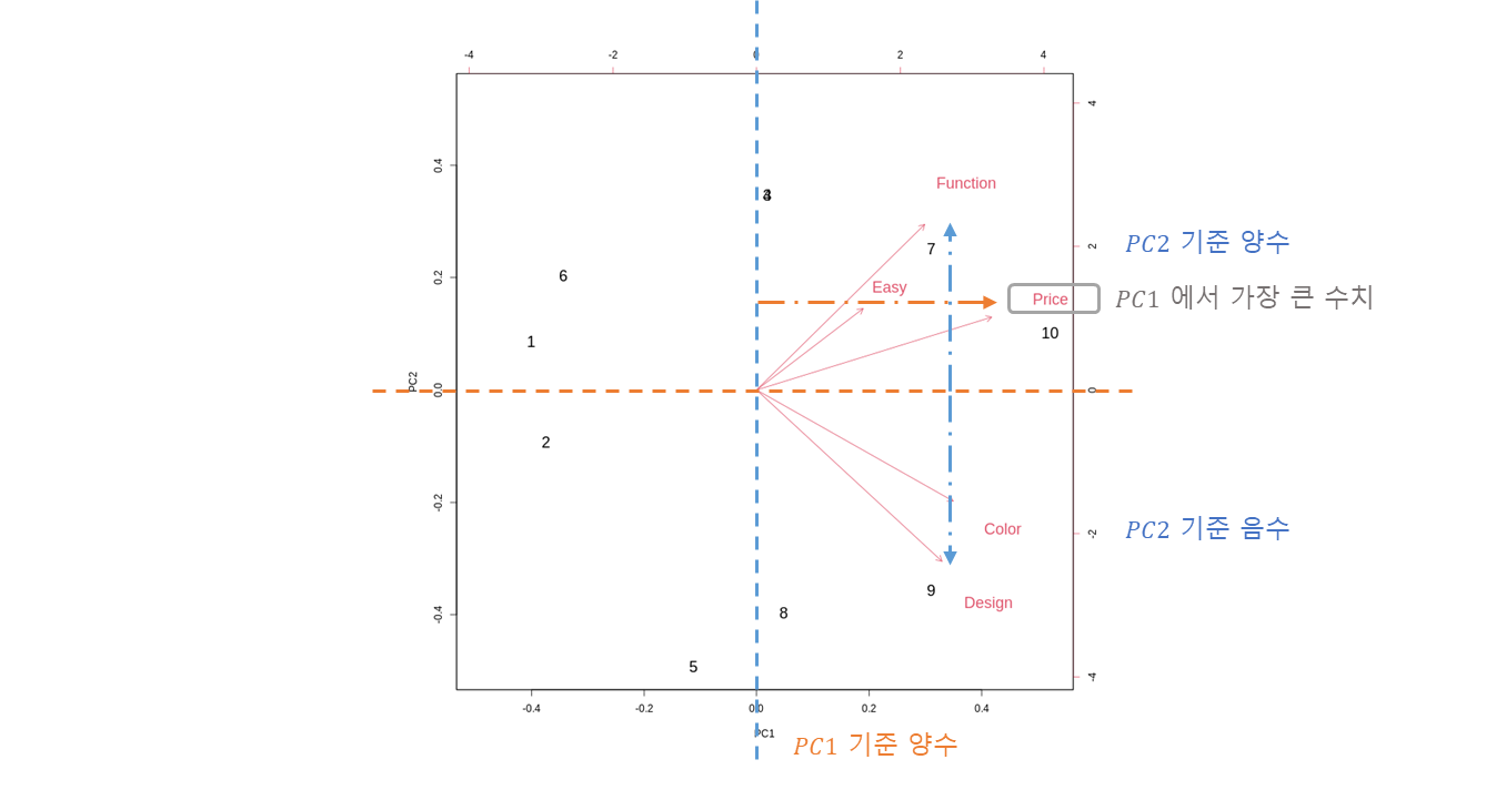
binary plot 으로 5차원의 데이터를 2차원으로 축소하여 시각화.
축소된 차원을 기준
: 첫 번째 주성분
: 두 번째 주성분
의 차원에서 원래 가지고 있던 5개의 차원의 Data 들이 어떻게 표현 되어 있는가를 역으로 표현.
-
Peason correlation matrix 에 기초하여 분석.
pca_model_corr = prcomp(Satis[,3:7], center=TRUE, scale=TRUE)
biplot(pca_model_corr, cex=c(1.5,1.5))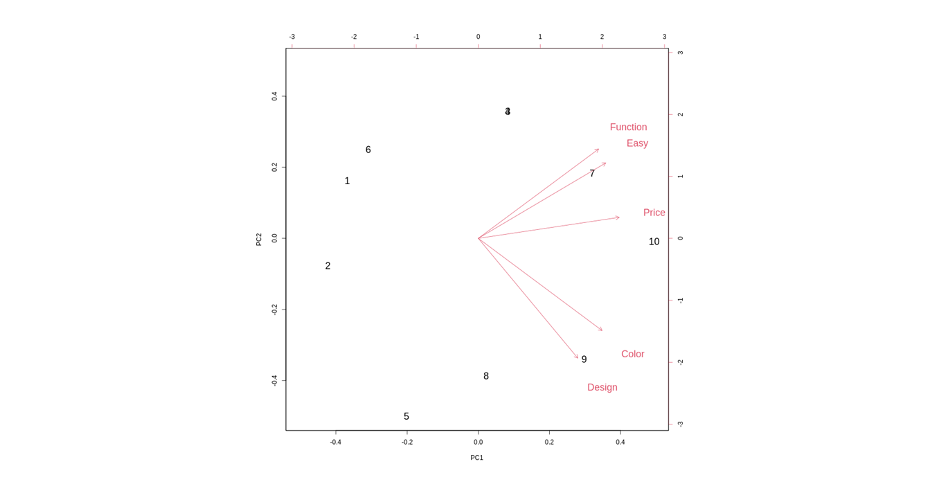
- 방향성은 같고, 크기가 각각 조금씩 평준화가 되었는데, 큰 차이는 없다.
- 모든 변수가 사이의 숫자로만 구성되어 있어, scale (unit, 단위) 가 같다.
- 따라서 correlation 을 기초로 하면 그 크기의 특징은 더 옅어진다. (분석 마다 다르다)
3. Result
그래서 주성분은 대체 몇개를 써야 하느냐?
- 전체 변이에 대한 공헌도
- 고유값의 크기 (Kaiser 의 규칙)
- eigenvalue, eigenvector
등은 다음에 다뤄보고, 시각적으로 찾을 수 있는 방법으로 확인해보자.
par(mfrow=c(2,2))
screeplot(pca_model, type='l', lwd=2)
screeplot(pca_model_corr, type='l', lwd=2)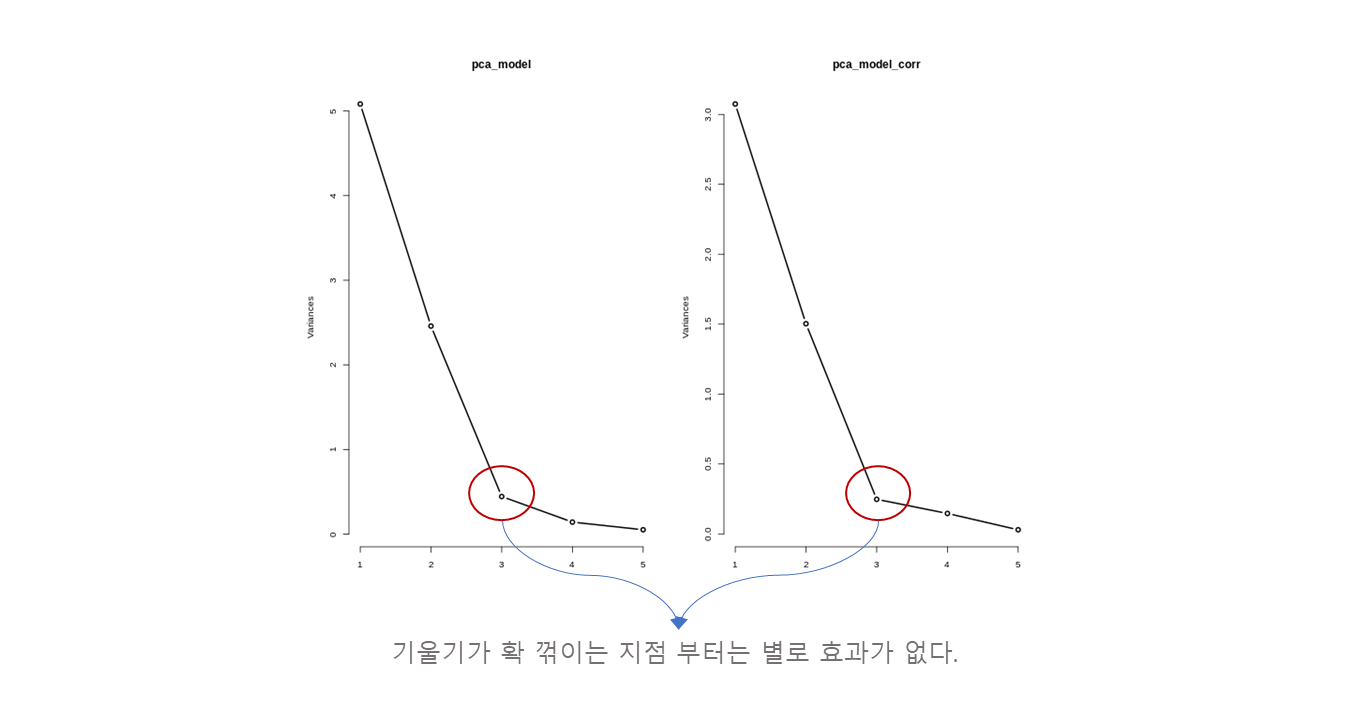
- 축은 주성분의 갯수.
- 축은 (분산, 변동).
- Covariance 기준에서 이 변동성을 5 만큼 가지고 있고, 이 변동성을 2.5 만큼 가지고 있다는 뜻.
- 부터는 작은 변동성을 가지고 있으므로, 설명력이 작다고 볼 수 있다.