Summary

Theorem: Composite Simpson's Rule

Let $f \in C^4[a, b], n$ be even, $h=(b-a) / n$, and $x_j=a+j h$, for each $j=0,1, \ldots, n$. There exists a $\mu \in(a, b)$ for which the Composite Simpson's rule for $n$ subintervals can be written with its error term as

$j=0,1, \ldots, n$ 각각에 대해 $f \in C^4[a, b], n$를 짝수, $h=(b-a)/n$ 및 $x_j=a+jh$로 하자. $n$ 하위 구간에 대한 복합 심슨의 규칙이 다음과 같은 오류 항으로 작성될 수 있는 $\mu \in(a, b)$가 있다.

Theorem: Composite Trapezoidal Rule

Let $f \in C^2[a, b], h=(b-a) / n$, and $x_j=a+j h$, for each $j=0,1, \ldots, n$. There exists a $\mu \in(a, b)$ for which the Composite Trapezoidal Rule for $n$ subintervals can be written with its error term as

$j=0,1, \ldots, n$ 각각에 대해 $f \in C^2[a, b], h=(b-a) /n$ 및 $x_j=a+jh$를 사용하자. $n$ 하위 구간에 대한 복합 사다리꼴 규칙을 다음과 같은 오류 용어로 작성할 수 있는 $\mu \in(a, b)$가 있다.

Theorem: Composite Midpoint Rule

Let $f \in C^2[a, b], n$ be even, $h=(b-a) /(n+2)$, and $x_j=a+(j+1) h$ for each $j=-1,0, \ldots, n+1$. There exists a $\mu \in(a, b)$ for which the Composite Midpoint rule for $n+2$ subintervals can be written with its error term as

$f \in C^2[a, b], n$이 짝수이고, $h=(b-a) /(n+2)$이며, $j=-1,0, \ldots, n+1$ 각각에 대해 $x_j=a+(j+1) h$라고 하자. $n+2$ 하위 구간에 대한 복합 중간점 규칙을 다음과 같은 오류 용어로 작성할 수 있는 $\mu \in(a, b)$가 있다.

A Motivating Example

Composite Numerical Integration: Motivating Example

Application of Simpson's Rule

Use Simpson's rule to approximate

and compare this to the results obtained by adding the Simpson's rule approximations for

and adding those for

Solution

Simpson's rule on $[0,4]$ uses $h=2$ and gives

The exact answer in this case is $e^4-e^0=53.59815$, and the error $-3.17143$ is far larger than we would normally accept.

Applying Simpson's rule on each of the intervals $[0,2]$ and $[2,4]$ uses $h=1$ and gives

The error has been reduced to $-0.26570$.

For the integrals on $[0,1],[1,2],[3,4]$, and $[3,4]$ we use Simpson's rule four times with $h=\frac{1}{2}$ giving

The error for this approximation has been reduced to $-0.01807$.

The Composite Simpson's Rule

Composite Numerical Integration: Simpson's Rule

To generalize this procedure for an arbitrary integral $\int_a^b f(x) d x$, choose an even integer $n$. Subdivide the interval $[a, b]$ into $n$ subintervals, and apply Simpson's rule on each consecutive pair of subintervals.

임의의 적분 $\int_a^b f(x) d x$에 대해 이 절차를 일반화하려면 짝수 정수 $n$을 선택한다. 간격 $[a, b]$를 $n$ 하위 간격으로 세분화하고, 각 연속 하위 간격 쌍에 대해 심슨의 규칙을 적용한다.

Construct the Formula \& Error Term

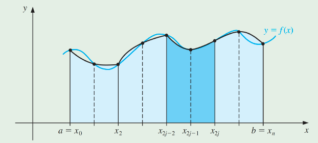
With $h=(b-a) / n$ and $x_j=a+j h$, for each $j=0,1, \ldots, n$, we have

for some $\xi_j$ with $x_{2 j-2}<\xi_j<x_{2 j}$, provided that $f \in C^4[a, b]$.

Using the fact that for each $j=1,2, \ldots,(n / 2)-1$ we have $f\left(x_{2 j}\right)$ appearing in the term corresponding to the interval $\left[x_{2 j-2}, x_{2 j}\right]$ and also in the term corresponding to the interval $\left[x_{2 j}, x_{2 j+2}\right]$, we can reduce this sum to

각 $j=1,2, \ldots, (n / 2)-1$에 대해 $f\left(x_{2 j}\right)$가 \left[x_{2 j-2], x_{2 j}\right] 간격에 해당하는 항과 $\left[x_{2 j}\right]$에 나타나는 것을 사용하여 우리는 이 합을 줄일 수 있다.

The error associated with this approximation is

이 근사치와 관련된 오차는 다음과 같다.

where $x_{2 j-2}<\xi_j<x_{2 j}$, for each $j=1,2, \ldots, n / 2$. If $f \in C^4[a, b]$, the Extreme Value Theorem csee theorem implies that $f^{(4)}$ assumes its maximum and minimum in $[a, b]$.

여기서 각 $j=1,2, \ldots, n / 2$에 대해 $x_{2j-2}<\xi_j<x_{2j}$. $f \in C^4[a,b]$일 경우, 극한값 정리는 $f^{(4)}$가 $[a,b]$에서 최대값과 최소값을 가정한다는 것을 암시한다.

Since

we have

and

By the Intermediate Value Theorem see theorem there is a $\mu \in(a, b)$ such that

Thus

or, since $h=(b-a) / n$,

These observations produce the following result.

Theorem: Composite Simpson's Rule

Let $f \in C^4[a, b], n$ be even, $h=(b-a) / n$, and $x_j=a+j h$, for each $j=0,1, \ldots, n$. There exists a $\mu \in(a, b)$ for which the Composite Simpson's rule for $n$ subintervals can be written with its error term as

$j=0,1, \ldots, n$ 각각에 대해 $f \in C^4[a, b], n$를 짝수, $h=(b-a)/n$ 및 $x_j=a+jh$로 하자. $n$ 하위 구간에 대한 복합 심슨의 규칙이 다음과 같은 오류 항으로 작성될 수 있는 $\mu \in(a, b)$가 있다.

Comments on the Formula \& Error Term

• Notice that the error term for the Composite Simpson's rule is $O\left(h^4\right)$, whereas it was $O\left(h^5\right)$ for the standard Simpson's rule.
• However, these rates are not comparable because, for the standard Simpson's rule, we have $h$ fixed at $h=(b-a) / 2$, but for Composite Simpson's rule we have $h=(b-a) / n$, for $n$ an even integer.
• This permits us to considerably reduce the value of $h$.
• The following algorithm uses the Composite Simpson's rule on $n$ subintervals. It is the most frequently-used general-purpose quadrature algorithm.

복합 심슨 규칙에 대한 오차항은 $O\left(h^4\right)$인 반면 표준 심슨 규칙에 대한 오차항은 $O\left(h^5\right)$였다.
그러나 표준 심슨 규칙의 경우 $h=(b-a)/2$로 고정되는 $h$를 가지지만 복합 심슨 규칙의 경우 $h=(b-a)/n$을 가지기 때문에 이러한 속도는 비교할 수 없다.
이를 통해 $h$의 가치를 상당히 줄일 수 있다.
다음 알고리즘은 $n$ 하위 간격에 대한 복합 심슨의 규칙을 사용한다. 가장 자주 사용되는 범용 직교 알고리즘이다.

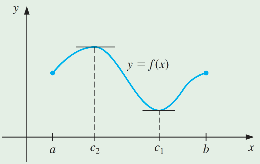
The Extreme Value Theorem

If $f \in C[a, b]$, then $c_1, c_2 \in[a, b]$ exist with $f\left(c_1\right) \leq f(x) \leq f\left(c_2\right)$, for all $x \in[a, b]$. In addition, if $f$ is differentiable on $(a, b)$, then the numbers $c_1$ and $c_2$ occur either at the endpoints of $[a, b]$ or where $f^{\prime}$ is zero.

$f \in C[a, b]$인 경우, 모든 $x \in[a, b]$에 대해 $f\left(c_1\right) \leq f(x) \leq f\left(c_2\right)$와 함께 $c_1, c_2 \in[a, b]$가 존재한다. 또한 $f$가 $(a, b)$에서 미분 가능한 경우 $c_1$과 $c_2$는 $[a, b]$의 끝점에서 발생하거나 $f^{\prime}$가 0인 경우이다.

The Composite Trapezoidal & Midpoint Rules

Composite Integration: Trapezoidal \& Midpoint Rules

Preamble

• The subdivision approach can be applied to any of the Newton-Cotes formulas.
• The extensions of the Trapezoidal and Midpoint rules will be presented without proof.
• The Trapezoidal rule requires only one interval for each application, so the integer $n$ can be either odd or even.
• For the Midpoint rule, however, the integer $n$ must be even.

사다리꼴 & 중간점 정리 서문
세분화 접근법은 임의의 뉴턴-코테스 공식에 적용될 수 있다.
사다리꼴 및 중간점 규칙의 확장은 증거 없이 제시될 것이다.
사다리꼴 규칙은 각 응용 프로그램에 대해 하나의 간격만 요구하므로 정수 $n$은 홀수이거나 짝수일 수 있다.
그러나 중간점 규칙의 경우 정수 $n$은 짝수여야 한다.

Note: The Trapezoidal rule requires only one interval for each application, so the integer $n$ can be either odd or even.

참고: 사다리꼴 규칙은 각 응용 프로그램에 대해 하나의 간격만 요구하므로 정수 $n$은 홀수이거나 짝수일 수 있다.

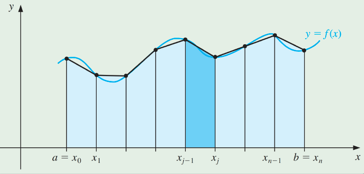
Theorem: Composite Trapezoidal Rule

Let $f \in C^2[a, b], h=(b-a) / n$, and $x_j=a+j h$, for each $j=0,1, \ldots, n$. There exists a $\mu \in(a, b)$ for which the Composite Trapezoidal Rule for $n$ subintervals can be written with its error term as

$j=0,1, \ldots, n$ 각각에 대해 $f \in C^2[a, b], h=(b-a) /n$ 및 $x_j=a+jh$를 사용하자. $n$ 하위 구간에 대한 복합 사다리꼴 규칙을 다음과 같은 error term으로 작성할 수 있는 $\mu \in(a, b)$가 있다.

Numerical Integration: Composite Midpoint Rule

Midpoint Rule (1-point open Newton-Cotes formula)

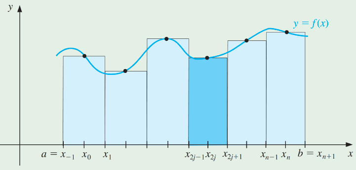
Theorem: Composite Midpoint Rule

Let $f \in C^2[a, b], n$ be even, $h=(b-a) /(n+2)$, and $x_j=a+(j+1) h$ for each $j=-1,0, \ldots, n+1$. There exists a $\mu \in(a, b)$ for which the Composite Midpoint rule for $n+2$ subintervals can be written with its error term as

$f \in C^2[a, b], n$이 짝수이고, $h=(b-a) /(n+2)$이며, $j=-1,0, \ldots, n+1$ 각각에 대해 $x_j=a+(j+1) h$라고 하자. $n+2$ 하위 구간에 대한 복합 중간점 규칙을 다음과 같은 error term으로 작성할 수 있는 $\mu \in(a, b)$가 있다.

Note: The Midpoint Rule requires two intervals for each application, so the integer $n$ must be even.

참고: 중간점 규칙은 각 응용 프로그램에 대해 두 개의 간격이 필요하므로 정수 $n$은 짝수여야 합니다.

Comparing the Composite Simpson & Trapezoidal Rules

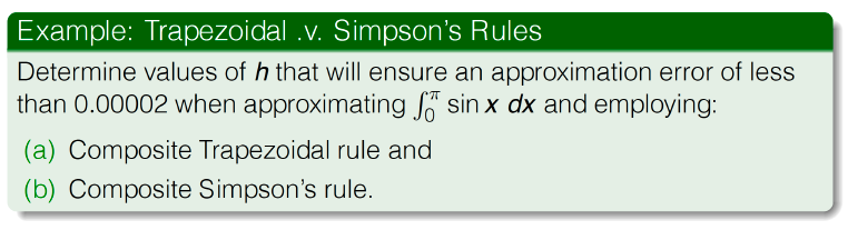
Composite Numerical Integration: Example

Composite Numerical Integration: Conclusion

• Composite Simpson's rule is the clear choice if you wish to minimize computation.
• For comparison purposes, consider the Composite Trapezoidal rule using $h=\pi / 18$ for the integral in the previous example.
• This approximation uses the same function evaluations as Composite Simpson's rule but the approximation in this case

  계산을 최소화하려면 컴포지트 심슨의 규칙이 확실한 선택이다.
  비교를 위해 이전 예의 적분에 $h=\pi / 18$를 사용하는 복합 사다리꼴 규칙을 고려해라.
  이 근사치는 컴포지트 심슨의 규칙과 동일한 함수 평가를 사용하지만 이 경우 근사치를 사용한다.

is accurate only to about $5 \times 10^{-3}$.

약 $5 \times 10^{-3}$까지만 정확하다.