4-7. Gaussian Quadrature

Summary

Legendre Polynomials Theorem

Suppose that $x_1, x_2, \ldots, x_n$ are the roots of the $n$th Legendre polynomial $P_n(\boldsymbol{x})$ and that for each $i=1,2, \ldots, n$, the numbers $c_i$ are defined by

$x_1, x_2, \ldots, x_n$이 $n$번째 르장드르 다항식 $P_n(x)$의 루트이고 각 $i=1,2, \ldots, n$에 대해 숫자 $c_i$는 다음과 같이 정의된다고 가정하자.

If $P(x)$ is any polynomial of degree less than $2 n$, then

$P(x)$가 $2 n$ 미만의 다항식이라면,

Gaussian Quadrature: Contrast with Newton-Cotes

비교

Features of a Newton-Cotes Formula

• The Newton-Cotes formulas were derived by integrating interpolating polynomials.
• The error term in the interpolating polynomial of degree $n$ involves the $(n+1)$ st derivative of the function being approximated, ...
• so a Newton-Cotes formula is exact when approximating the integral of any polynomial of degree less than or equal to $n$.

뉴턴-코테스 공식은 보간 다항식을 통합하여 도출되었다.
차수 $n$의 보간 다항식의 오차 항은 근사되는 함수의 $(n+1)$st 도함수를 포함한다.
따라서 뉴턴-코츠 공식은 $n$ 이하의 다항식의 적분을 근사할 때 정확하다.

• All the Newton-Cotes formulas use values of the function at equally-spaced points.
• This restriction is convenient when the formulas are combined to form the composite rules which we considered earlier, ...
• but it can significantly decrease the accuracy of the approximation.

모든 뉴턴-코츠 공식은 동일한 간격의 점에서 함수의 값을 사용한다.
이 제한사항은 공식이 복합 규칙을 형성하기 위해 결합될 때 편리하다.
그러나 근사치의 정확도를 크게 떨어뜨릴 수 있다.

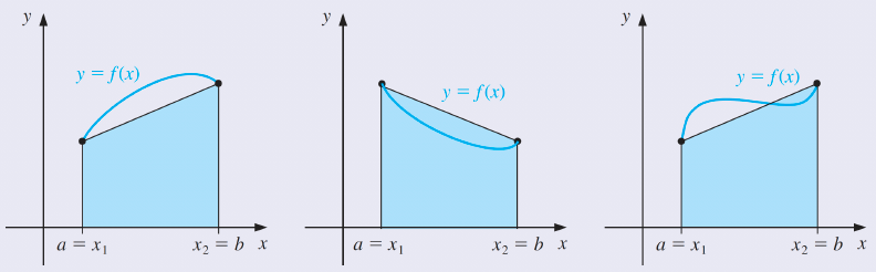
Consider, for example, the Trapezoidal rule applied to determine the integrals of the functions whose graphs are as shown.

It approximates the integral of the function by integrating the linear function that joins the endpoints of the graph of the function.

함수의 그래프의 끝점을 연결하는 선형 함수를 통합하여 함수의 적분을 근사한다.

Gaussian Integration: Optimal integration points

But this is not likely the best line for approximating the integral. Lines such as those shown below would likely give much better approximations in most cases.

그러나 이것은 적분을 근사하는 데 가장 좋은 선은 아닐 것이다. 아래 표시된 것과 같은 선은 대부분의 경우 훨씬 더 나은 근사치를 제공할 수 있다.

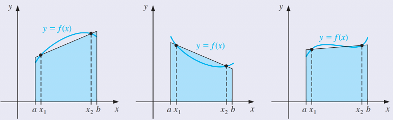
Gaussian quadrature chooses the points for evaluation in an optimal, rather than equally-spaced, way.

가우스 직교법은 평가를 위해 동일한 간격의 포인트가 아닌 최적의 방식으로 선택된다.

Gaussian Quadrature: Introduction

Choice of Integration Nodes

• The nodes $\boldsymbol{x}_1, x_2, \ldots, x_n$ in the interval $[a, b]$ and coefficients $c_1, c_2, \ldots, c_n$, are chosen to minimize the expected error obtained in the approximation

  $[a, b]$ 간격의 노드 $\boldsymbol{x}_1, x_2, \ldots, x_n$과 계수 $c_1, c_2, \ldots, c_n$은 근사치에서 얻은 예상 오류를 최소화하기 위해 선택된다.

• To measure this accuracy, we assume that the best choice of these values produces the exact result for the largest class of polynomials, ...

• that is, the choice that gives the greatest degree of precision.

  이 정확도를 측정하기 위해, 우리는 이러한 값들의 최선의 선택이 가장 큰 종류의 다항식에 대한 정확한 결과를 생성한다고 가정한다.
  즉, 가장 높은 정밀도를 제공하는 선택이다.

• The coefficients $c_1, c_2, \ldots, c_n$ in the approximation formula are arbitrary, and the nodes $\boldsymbol{x}_1, \boldsymbol{x}_2, \ldots, \boldsymbol{x}_n$ are restricted only by the fact that they must lie in $[a, b]$, the interval of integration.

• This gives us $2 n$ parameters to choose.

  근사 공식의 계수 $c_1, c_2, \ldots, c_n$은 임의이며, 노드 $\boldsymbol{x}_1, \boldsymbol{x}_2, \ldots, \boldsymbol{x}_n$은 통합 간격 $[a, b]$에 있어야 한다는 사실에 의해서만 제한된다.
  이것은 선택할 수 있는 $2n$ 매개 변수를 제공한다.

• If the coefficients of a polynomial are considered parameters, the class of polynomials of degree at most $2 n-1$ also contains $2 n$ parameters.

• This, then, is the largest class of polynomials for which it is reasonable to expect a formula to be exact.

• With the proper choice of the values and constants, exactness on this set can be obtained.

  다항식의 계수를 매개 변수로 간주하면 최대 $2n-1$의 다항식 클래스에도 $2n$ 매개 변수가 포함됩니다.
  따라서, 이것은 공식이 정확할 것으로 예상하는 것이 합리적인 다항식의 가장 큰 종류이다.
  값과 상수의 적절한 선택을 통해 이 집합에 대한 정확성을 얻을 수 있다.

Gaussian Quadrature: Illustration (n=2)

Formula when n=2 on [-1,1]

Gaussian Quadrature: Legendre Polynomials

An Alternative Method of Derivation

• We will consider an approach which generates more easily the nodes and coefficients for formulas that give exact results for higher-degree polynomials.
• This will be achieved using a particular set of orthogonal polynomials (functions with the property that a particular definite integral of the product of any two of them is 0 ).

우리는 고차 다항식에 대한 정확한 결과를 제공하는 공식에 대한 노드와 계수를 더 쉽게 생성하는 접근법을 고려할 것이다.
이것은 특정한 직교 다항식 집합을 사용하여 달성될 것이다. (이들 중 임의의 두 곱의 특정 유한 적분이 0인 성질을 갖는 함수).

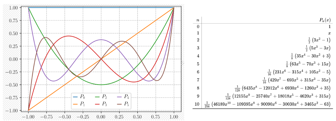
• This set is the is the Legendre polynomials, a collection $\left\{P_0(x), P_1(x), \ldots, P_n(x), \ldots,\right\}$ with properties:
  (1) For each $n, P_n(x)$ is a monic polynomial of degree $n$.
  (2) $\int_{-1}^1 P(x) P_n(x) d x=0$ whenever $P(x)$ is a polynomial of degree less than $n$.

The first few Legendre Polynomials

$P_3(x)=x^3-\frac{3}{5} x \quad$ and $\quad P_4(x)=x^4-\frac{6}{7} x^2+\frac{3}{35}$

• The roots of these polynomials are distinct, lie in the interval $(-1,1)$, have a symmetry with respect to the origin, and, most importantly,
• they are the correct choice for determining the parameters that give us the nodes and coefficients for our quadrature method.

  이러한 다항식의 근은 구별되며, $(-1,1)$ 간격에 있으며, 원점에 대한 대칭을 가지고 있으며, 가장 중요한 것은,
  그들은 우리에게 직교법에 대한 노드와 계수를 제공하는 매개 변수를 결정하기 위한 올바른 선택이다.

Gaussian Quadrature: Legendre Polynomials

The nodes $x_1, x_2, \ldots, x_n$ needed to produce an integral approximation formula that gives exact results for any polynomial of degree less than $2 n$ are the roots of the $n$ th-degree Legendre polynomial.

$2n$ 미만의 모든 다항식에 대한 정확한 결과를 제공하는 적분 근사 공식을 생성하는 데 필요한 노드 $x_1, x_2, \ldots, x_n$은 $n$번째 차수 르장드르 다항식의 루트이다.

Theorem

Suppose that $x_1, x_2, \ldots, x_n$ are the roots of the $n$th Legendre polynomial $P_n(\boldsymbol{x})$ and that for each $i=1,2, \ldots, n$, the numbers $c_i$ are defined by

$x_1, x_2, \ldots, x_n$이 $n$번째 르장드르 다항식 $P_n(\boldsymbol{x})$의 루트이고 각 $i=1,2, \ldots, n$에 대해 숫자 $c_i$는 다음과 같이 정의된다고 가정하자.

If $P(x)$ is any polynomial of degree less than $2 n$, then

$P(x)$가 $2 n$ 미만의 다항식이라면,

Proof

• Let us first consider the situation for a polynomial $P(x)$ of degree less than $n$.

• Re-write $P(x)$ in terms of $(n-1)$ st Lagrange coefficient polynomials with nodes at the roots of the $n$th Legendre polynomial $P_n(x)$

  먼저 $n$ 미만의 다항식 $P(x)$의 상황을 고려해보자.
  $n$th Legendre 다항식 $P_n(x)$의 루트에 노드가 있는 $(n-1)$ st Lagrange 계수 다항식의 관점에서 $P(x)$를 다시 쓴다.

• Let us first consider the situation for a polynomial $P(x)$ of degree less than $n$.

• Re-write $P(x)$ in terms of $(n-1)$ st Lagrange coefficient polynomials with nodes at the roots of the $n$th Legendre polynomial $P_n(x)$

• The error term for this representation involves the $n$th derivative of $P(x)$

• Since $P(x)$ is of degree less than $n$, the $n$th derivative of $P(x)$ is 0 , and this representation of is exact. So

  먼저 $n$ 미만의 다항식 $P(x)$의 상황을 고려해보자.
  $n$th Legendre 다항식 $P_n(x)$의 루트에 노드가 있는 $(n-1)$ st Lagrange 계수 다항식의 관점에서 $P(x)$를 다시 쓴다.
  이 표현의 오류 항은 $P(x)$의 $n$번째 도함수를 포함한다.
  $P(x)$는 $n$보다 작기 때문에 $P(x)$의 $n$번째 도함수는 0이며, 이 표현은 정확하다.

Therefore

Hence the result is true for polynomials of degree less than $n$.

따라서 결과는 $n$ 미만의 다항식의 경우 참이다.

• Now consider a polynomial $P(x)$ of degree at least $n$ but less than $2 n$
• Divide $P(x)$ by the $n$th Legendre polynomial $P_n(x)$.
• This gives two polynomials $Q(x)$ and $R(x)$, each of degree less than $n$, with
  $P(x)=Q(x) P_n(x)+R(x)$
• Note that $x_i$ is a root of $P_n(x)$ for each $i=1,2, \ldots, n$, so we have
  $P\left(x_i\right)=Q\left(x_i\right) P_n\left(x_i\right)+R\left(x_i\right)=R\left(x_i\right)$
• We now invoke the unique power of the Legendre polynomials.

이제 $n$ 이상 $2n$ 미만의 다항식 $P(x)$를 고려하십시오.
$P(x)$를 $n$th Legendre 다항식 $P_n(x)$로 나눈다.
이것은 두 개의 다항식 $Q(x)$와 $R(x)$을 제공하며, 각 차수는 $n$ 미만이다.

$x_i$는 각 $i=1,2, \ldots,n$에 대한 $P_n(x)$의 루트이기 때문에 다음과 같은 값을 갖는다.

이제 우리는 르장드르 다항식의 고유한 힘을 호출한다.

First, the degree of the polynomial $Q(x)$ is less than $n$, so (by the Legendre orthogonality property),

Then, since $R(x)$ is a polynomial of degree less than $n$, the opening argument implies that

첫째, 다항식 $Q(x)$의 정도가 $n$ 미만이기 때문에 (레전드 직교성 속성에 의해),

그렇다면, $R(x)$은 $n$ 미만의 다항식이기 때문에, 오프닝 인수는 다음을 암시한다.

Putting these facts together verifies that the formula is exact for the polynomial $P(x)$ :

이러한 사실을 종합하면 공식이 다항식 $P(x)$에 대해 정확하다는 것을 확인할 수 있다.

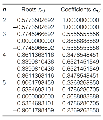
Gaussian Quadrature: Roots \& Coefficients

The constants $c_i$ needed for the quadrature rule can be generated from the equation given in the theorem:

구법칙에 필요한 상수 $c_i$는 정리에 주어진 방정식에서 생성될 수 있다.

but both these constants and the roots of the Legendre polynomials are extensively tabulated.

그러나 이러한 상수와 라장드르 다항식의 근은 모두 광범위하게 표로 작성되었다.

The following table lists these values for $n=2,3,4$, and 5 .

다음 표에는 $n=2,3,4$ 및 5에 대한 값이 나열되어 있습다.

Gaussian Quadrature: Legendre Polynomials

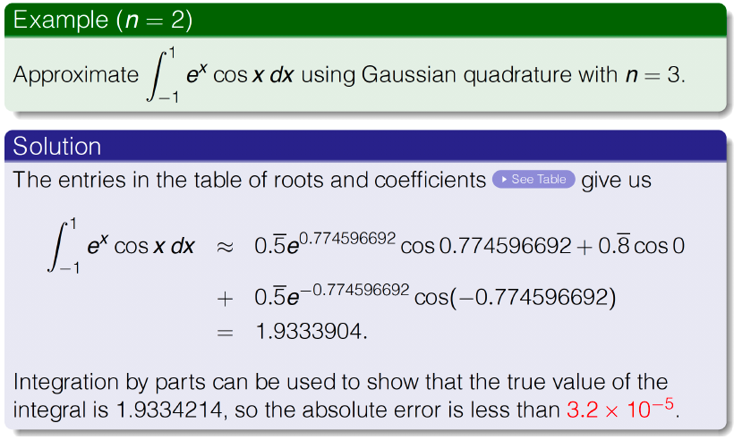
Example (n=2)

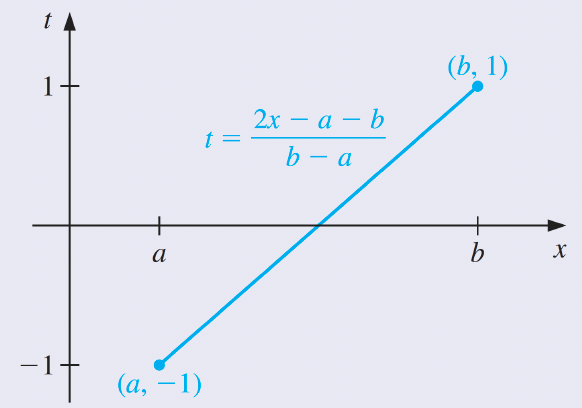
Gaussian Quadrature on Arbitrary Intervals

Transform the Interval of Integration to $[-1,1]$

An integral $\int_a^b f(x) d x$ over an arbitrary $[a, b]$ can be transformed into an integral over $[-1,1]$ by using the change of variables

임의의 $[a, b]$에 대한 적분 $\int_a^b f(x) d x$는 변수 변경을 사용하여 $[-1,1]$에 대한 적분으로 변환할 수 있다.

This permits Gaussian quadrature to be applied to any interval $[a, b]$, because

이것은 가우스 직교법을 임의의 간격 $[a, b]$에 적용할 수 있게 해준다, 왜냐하면

Mapping Interval [a,b] onto [-1,1]

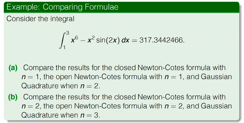
Example: Comparing Formulae (31p)

Open & Closed Newton-Cotes Formulae $(n=1)$

• Closed $n=1$ : Trapezoidal Rule:

  $\int_{x_0}^{x_1} f(x) d x=\frac{h}{2}\left[f\left(x_0\right)+f\left(x_1\right)\right]-\frac{h^3}{12} f^{\prime \prime}(\xi)$

  where $x_0<\xi<x_1$.

• Open $n=1$ :

  $\int_{x_{-1}}^{x_2} f(x) d x=\frac{3 h}{2}\left[f\left(x_0\right)+f\left(x_1\right)\right]+\frac{3 h^3}{4} f^{\prime \prime}(\xi)$

  where $x_{-1}<\xi<x_2$.

• $n=0$ : Midpoint Rule:

  $\int_{x_{-1}}^{x_1} f(x) d x=2 h f\left(x_0\right)+\frac{h^3}{3} f^{\prime \prime}(\xi)$

  where $x_{-1}<\xi<x_1$.

• Open $n=2$

  $\int_{x_{-1}}^{x_3} f(x) d x=\frac{4 h}{3}\left[2 f\left(x_0\right)-f\left(x_1\right)+2 f\left(x_2\right)\right]+\frac{14 h^5}{45} f^{(4)}(\xi)$

  where $x_{-1}<\xi<x_3$.