함수의 근사
데이터가 주어져 있을 때, 데이터가 어떤 함수로부터 나왔을까?

Weierstrass Approximation Theorem

Algebraic Polynomials

One of the most useful and well-known classes of functions mapping the set of real numbers into itself is the algebraic polynomials, the set of functions of the form

where $n$ is a nonnegative integer and $a_0, \ldots, a_n$ are real constants.

Algebraic Polynomials (Cont'd)

• One reason for their importance is that they uniformly approximate continuous functions.
• By this we mean that given any function, defined and continuous on a closed and bounded interval, there exists a polynomial that is as "close" to the given function as desired.
• This result is expressed precisely in the Weierstrass Approximation Theorem.

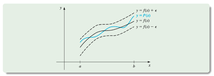
Weierstrass Approximation Theorem

Suppose that $f$ is defined and continuous on $[a, b]$. For each $\epsilon>0$, there exists a polynomial $P(x)$, with the property that

Benefits of Algebraic Polynomials

• Another important reason for considering the class of polynomials in the approximation of functions is that the derivative and indefinite integral of a polynomial are easy to determine and are also polynomials.
• For these reasons, polynomials are often used for approximating continuous functions.

Inaccuracy of Taylor Polynomials

The Lagrange Polynomial: Taylor Polynomials

Interpolating with Taylor Polynomials

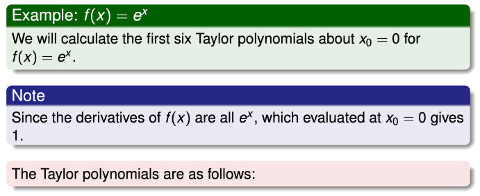
• The Taylor polynomials are described as one of the fundamental building blocks of numerical analysis.
• Given this prominence, you might expect that polynomial interpolation would make heavy use of these functions.
• However this is not the case.
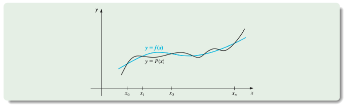
• The Taylor polynomials agree as closely as possible with a given function at a specific point, but they concentrate their accuracy near that point.
• A good interpolation polynomial needs to provide a relatively accurate approximation over an entire interval, and Taylor polynomials do not generally do this.

Footnotes

• For the Taylor polynomials, all the information used in the approximation is concentrated at the single number $x_0$, so these polynomials will generally give inaccurate approximations as we move away from $x_0$.
• This limits Taylor polynomial approximation to the situation in which approximations are needed only at numbers close to $x_0$.
• For ordinary computational purposes, it is more efficient to use methods that include information at various points.
• The primary use of Taylor polynomials in numerical analysis is not for approximation purposes, but for the derivation of numerical techniques and error estimation.

Example

Constructing the Lagrange Polynomial

The Lagrange Polynomial: The Linear Case

Polynomial Interpolation

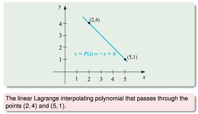
• The problem of determining a polynomial of degree one that passes through the distinct points
  $\left(x_0, y_0\right) \text { and }\left(x_1, y_1\right)$
  is the same as approximating a function $f$ for which
  $f\left(x_0\right)=y_0 \quad \text { and } f\left(x_1\right)=y_1$
  by means of a first-degree polynomial interpolating, or agreeing with, the values of $f$ at the given points.
• Using this polynomial for approximation within the interval given by the endpoints is called polynomial interpolation.

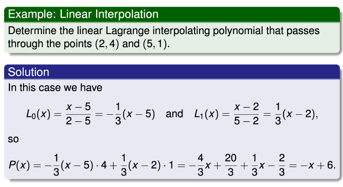
Define the functions

Definition

The linear Lagrange interpolating polynomial though $\left(x_0, y_0\right)$ and $\left(x_1, y_1\right)$ is

Note that

which implies that

and

So $P$ is the unique polynomial of degree at most 1 that passes through $\left(x_0, y_0\right)$ and $\left(x_1, y_1\right)$

Example

The Lagrange Polynomial: Degree $n$ Construction

To generalize the concept of linear interpolation, consider the construction of a polynomial of degree at most $n$ that passes through the $n+1$ points

The Lagrange Polynomial: The General Case

Constructing the Degree $n$ Polynomial

• We first construct, for each $k=0,1, \ldots, n$, a function $L_{n, k}(x)$ with the property that $L_{n, k}\left(x_i\right)=0$ when $i \neq k$ and $L_{n, k}\left(x_k\right)=1$.
• To satisfy $L_{n, k}\left(x_i\right)=0$ for each $i \neq k$ requires that the numerator of $L_{n, k}(x)$ contain the term
  $\left(x-x_0\right)\left(x-x_1\right) \cdots\left(x-x_{k-1}\right)\left(x-x_{k+1}\right) \cdots\left(x-x_n\right) .$
• To satisfy $L_{n, k}\left(x_k\right)=1$, the denominator of $L_{n, k}(x)$ must be this same term but evaluated at $x=x_k$.
• Thus
  $L_{n, k}(x)=\frac{\left(x-x_0\right) \cdots\left(x-x_{k-1}\right)\left(x-x_{k+1}\right) \cdots\left(x-x_n\right)}{\left(x_k-x_0\right) \cdots\left(x_k-x_{k-1}\right)\left(x_k-x_{k+1}\right) \cdots\left(x_k-x_n\right)} \text {. }$
  

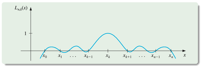
Theorem: $\boldsymbol{n}$-th Lagrange interpolating polynomial

If $x_0, x_1, \ldots, x_n$ are $n+1$ distinct numbers and $f$ is a function whose values are given at these numbers, then a unique polynomial $P(x)$ of degree at most $n$ exists with

This polynomial is given by

where, for each $k=0,1, \ldots, n, L_{n, k}(x)$ is defined as follows:

Definition of $L_{n, k}(x)$

We will write $L_{n, k}(x)$ simply as $L_k(x)$ when there is no confusion as to its degree.

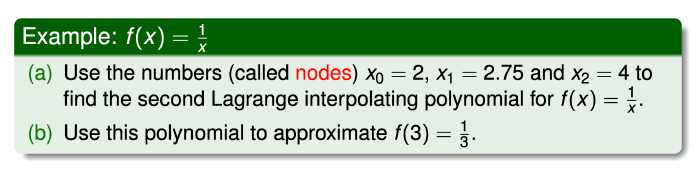
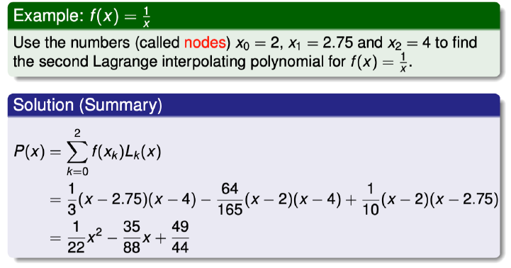
Example: Second-Degree Lagrange Interpolating Polynomial

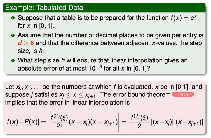
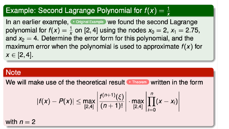
Interpolating Polynomial Error Bound

The Lagrange Polynomial: Theoretical Error Bound

Theorem

Suppose $x_0, x_1, \ldots, x_n$ are distinct numbers in the interval $[a, b]$ and $f \in C^{n+1}[a, b]$. Then, for each $x$ in $[a, b]$, a number $\xi(x)$ (generally unknown) between $x_0, x_1, \ldots, x_n$, and hence in $(a, b)$, exists with

where $P(x)$ is the interpolating polynomial given by

Error Bound: Proof (skip)

Generalized Rolle's Theorem

Suppose $f \in C[a, b]$ is $n$ times differentiable on $(a, b)$. If

at the $n+1$ distinct numbers $a \leq x_0<x_1<\ldots<x_n \leq b$, then a number $c$ in $\left(x_0, x_n\right)$, and hence in $(a, b)$, exists with

Example: 2nd Lagrange Interpolating Polynomial Error Bound

Example: Interpolaing Polynomial Error for Tabulated Data