📆개발 시기
2022.06.06.-2022.06.08.
📝개발 목적
사람 얼굴 이미지 파일 15개, 컴퓨터 이미지 파일 15개를 제공하여 EfficientNet B0 모델로 학습하고,
예측용으로 제공되는 10장의(사람 5장 + 컴퓨터 5장) 이미지 데이터 중 컴퓨터인 것만 인쇄하는 프로그램이다.
📕준비
-
학습 이미지: 사람 이미지 15장, 컴퓨터 이미지 15장 -
예측 이미지: 사람 이미지 5장, 컴퓨터 이미지 5장 -
모델: EfficientNet B0
학습과 예측 이미지인 총 20장의 이미지는 Github에 미리 올려놓고 수행
🔍실험 환경
OS : Windows 10
CPU : Intel(R) Core(TM) i7-6700 CPU
RAM : 16GB
GPU : RTX 2060
Jupyter
📃실험 준비
import matplotlib.pyplot as plt
import numpy as np
from skimage.io import imread # 이미지를 읽어 들인다
from skimage.transform import resize
url = 깃허브 주소
computer_images = []
for i in range(15):
file = url + 'img{0:02d}.jpg'.format(i+1)
img = imread(file)
img = resize(img, (224,224))
computer_images.append(img)
def plot_images(nRow, nCol, img):
fig = plt.figure()
fig, ax = plt.subplots(nRow, nCol, figsize = (nCol,nRow))
for i in range(nRow):
for j in range(nCol):
if nRow <= 1: axis = ax[j]
else: axis = ax[i, j]
axis.get_xaxis().set_visible(False)
axis.get_yaxis().set_visible(False)
axis.imshow(img[i*nCol+j])
plot_images(3,5, computer_images)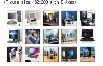 컴퓨터 이미지 15장을 읽어 들인다.
그 후 plot_images 함수를 통해 시각적으로 이미지를 보여준다.
url = url 주소
human_images = []
for i in range(15):
file = url + 'img{0:02d}.jpg'.format(i+1)
img = imread(file,plugin='matplotlib')
img = resize(img, (224,224))
human_images.append(img)
plot_images(3,5, human_images)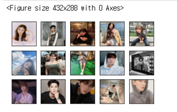 사람 이미지를 깃허브로부터 읽고
 human_images 배열에 저장한다.
마찬가지로 plot_images 함수를 통하여 이미지를 출력한다
X = computer_images+ human_images
y = [ [1,0] ]* len(computer_images) + [ [0,1] ] * len(human_images)
X = np.array(X)
y = np.array(y)
print(X.shape, y.shape)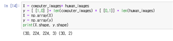
computer 데이터셋의 배열과 human 데이터셋의 배열을 취합하여 X로 지정한다.
y는 여러 X들로 인해 정해지는 값이다.
💻EfficientNet-B0
from sklearn.model_selection import StratifiedShuffleSplit
import cv2
from skimage.transform import resize
import numpy as np
import pandas as pd
import matplotlib.pyplot as plt
%matplotlib inline
from pylab import rcParams
from sklearn.metrics import accuracy_score, confusion_matrix, classification_report
from keras.callbacks import Callback, EarlyStopping, ReduceLROnPlateau
import tensorflow as tf
import keras
from keras.models import Sequential, load_model
from keras.layers import Dropout, Dense, GlobalAveragePooling2D
from keras.optimizers import Adam
from tensorflow.keras.applications import EfficientNetB0
height = 224
width = 224
channels = 3
input_shape = (height, width, channels)
efnb0 = EfficientNetB0(weights='imagenet', include_top=False, input_shape=input_shape, classes=2)
model = Sequential()
model.add(efnb0)
model.add(GlobalAveragePooling2D())
model.add(Dropout(0.5))
model.add(Dense(2, activation='softmax'))
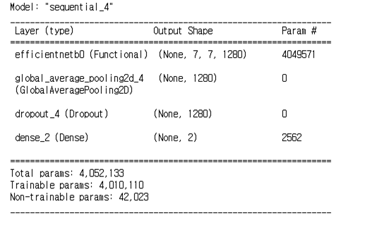
model.summary()사전 훈련된 EfficientNet-B0 모델을 사용하는 코드이다.
해당 모델은 총 4049571개의 훈련 가능한 매개변수가 있다.
📌학습
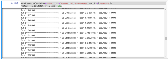
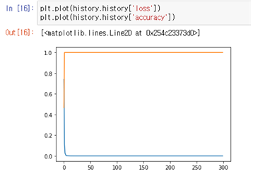
model.compile(optimizer='adam', loss='categorical_crossentropy', metrics=['accuracy'])
history = model.fit(X, y, epochs = 300)
EfficientNet - B0 모델을 300번 학습시킨다.
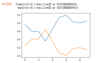
결과 그래프
test_result = model.predict(test_images)
plt.plot(test_result)
테스트 이미지에 대한 예측 후 결과 그래프를 나타낸다
📰출력 결과
예측 이미지 데이터셋
예측 이미지 데이터셋은 사람 5장, 컴퓨터 5장으로 구성된다.
url = 테스트 데이터 url

test_images = []

for i in range(10):
    file = url + 'img{0:02d}.jpg'.format(i+1)
    img = imread(file,plugin='matplotlib')
    img = resize(img, (224,224))
    test_images.append(img)

test_images = np.array(test_images)
plot_images(2, 5, test_images)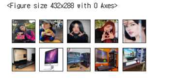
테스트 결과
fig = plt.figure()
fig, ax = plt.subplots(2,5, figsize = (10,4))
for i in range(2):
    for j in range(5):
        ax[i, j].get_xaxis().set_visible(False)
        ax[i, j].get_yaxis().set_visible(False)
        if test_result[i*5+j][0] > 0.8:
            ax[i, j].imshow(test_images[i*5+j],interpolation='nearest')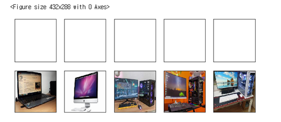
최종 예측 이미지 데이터로 테스트한 결과(정확도 0.8 이상인 결과)
🎯성능
test_result = model.predict(test_images)
plt.plot(test_result)
학습된 모델의 정확도 및 손실율 그래프를 나타낸다.
📂고찰
정확도 및 손실율 그래프를 통해 눈으로 정확도를 확인할 수 있으며, 도출된 결과를 통해 컴퓨터인 것만 인쇄하였으므로 학습이 잘 된것을 확인 가능
🧸담당 역할
- GitHub의 컴퓨터 이미지 15장을 읽고,
plot_images함수로 이미지 출력 - 사람의 이미지를 깃허브로부터 읽고 human_images 배열에 저장
- computer 데이터셋의 배열과 human 데이터셋 배열을 취합하여 X로 지정
- 사전 훈련된 EfficientNet-B0를 사용해 300번 학습
- 예측 이미지 데이터셋을 구성 후 테스트
📚참고문헌
[1]EfficientNet B0 참고문헌 :
https://www.tensorflow.org/api_docs/python/tf/keras/applications/efficientnet/EfficientNetB0
[2]2-(5)의 참고 문헌 :
https://towardsdatascience.com/cifar-100-transfer-learning-using-efficientnet-ed3ed7b89af2