cs231n 과제2 Q4- Convolutional Neural Networks

  이번 과제에서는 CNN을 구현해보는 것을 목표로 한다. CNN이 어떻게 구성되고 계산되는지는 알고 있지만, 막상 이렇게 구현하려고 하니 어떻게 코드를 쓸지 막막했다. 그렇기 때문에 이번에는 그림을 그려가면서 내가 이해했던 과정들을 소개하려고 한다.

1. conv_forward_naive 함수

def conv_forward_naive(x, w, b, conv_param):
    out = None
    ###########################################################################
    # TODO: Implement the convolutional forward pass.                         #
    # Hint: you can use the function np.pad for padding.                      #
    ###########################################################################
    # *****START OF YOUR CODE (DO NOT DELETE/MODIFY THIS LINE)*****
    stride=conv_param['stride']
    pad=conv_param['pad']
    N=x.shape[0]
    F=w.shape[0]
    H=x.shape[2]
    W=x.shape[3]
    HH=w.shape[2]
    WW=w.shape[3]
    H_out= 1+ (H+2*pad-HH)//stride
    W_out= 1+ (W+2*pad-WW)//stride
    out = np.zeros([N,F,H_out,W_out])
    pad_width=[(0,0),(0,0),(pad,pad),(pad,pad)]
    x_pad= np.pad(x,pad_width,mode='constant') #has shape (N,C,H+2*pad,W+2*pad)
    for i in range(N): #iterate for N inputs.
      for j in range(F): # number fo filters
        for p in range(H_out):
          for q in range(W_out):
             H_now=p*stride
             W_now=q*stride
             out[i,j,p,q]=np.sum(x_pad[i,:,H_now:H_now+HH,W_now:W_now+WW]*w[j,:,:,:])+b[j] #elementwise multiplication.
    # *****END OF YOUR CODE (DO NOT DELETE/MODIFY THIS LINE)*****
    ###########################################################################
    #                             END OF YOUR CODE                            #
    ###########################################################################
    cache = (x, w, b, conv_param)
    return out, cache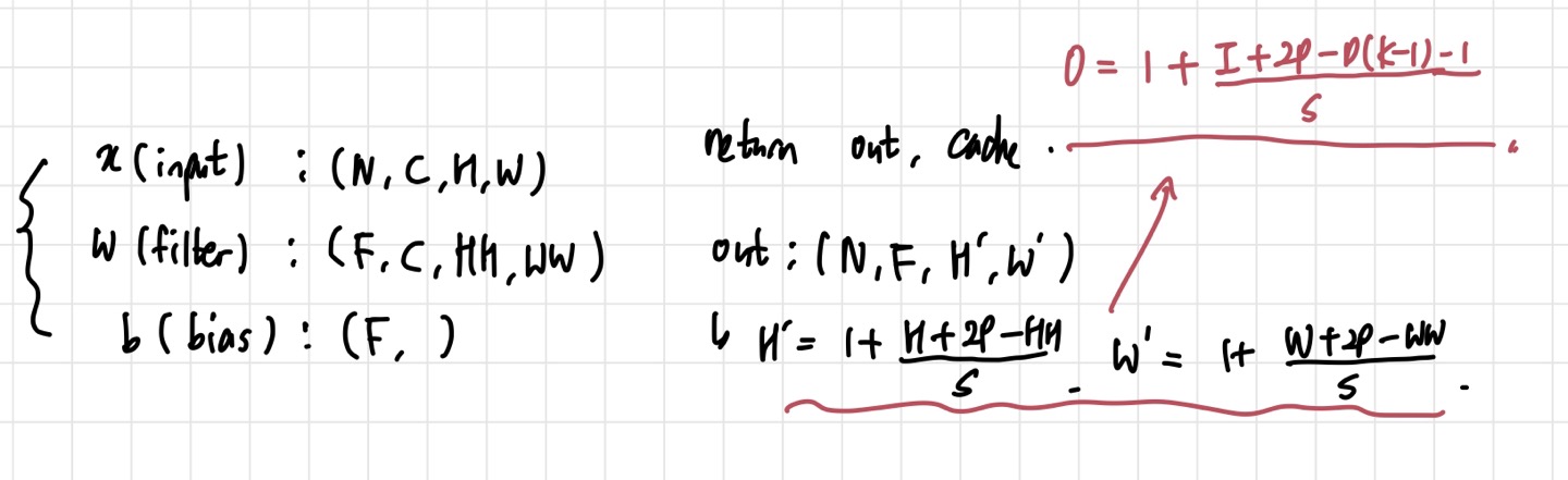

  함수에 주어지는 $x,w,b$ 값들의 shape은 위의 사진과 같다. $N$은 input 개수, $C$는 채널 수, $H,W$는 각각 input height와 width를 의미한다. $F$는 filter의 개수를 의미하고, $HH$와 $WW$는 filter의 height와 width를 뜻한다. cs231n에서 배웠듯이, filter의 개수= output channel수 이므로 out은 $F$개의 channel들을 갖게 된다. $H'$와 $W'$는 이전에 배운 공식(위 사진에서 빨간 식)을 통해 얻을 수 있다.

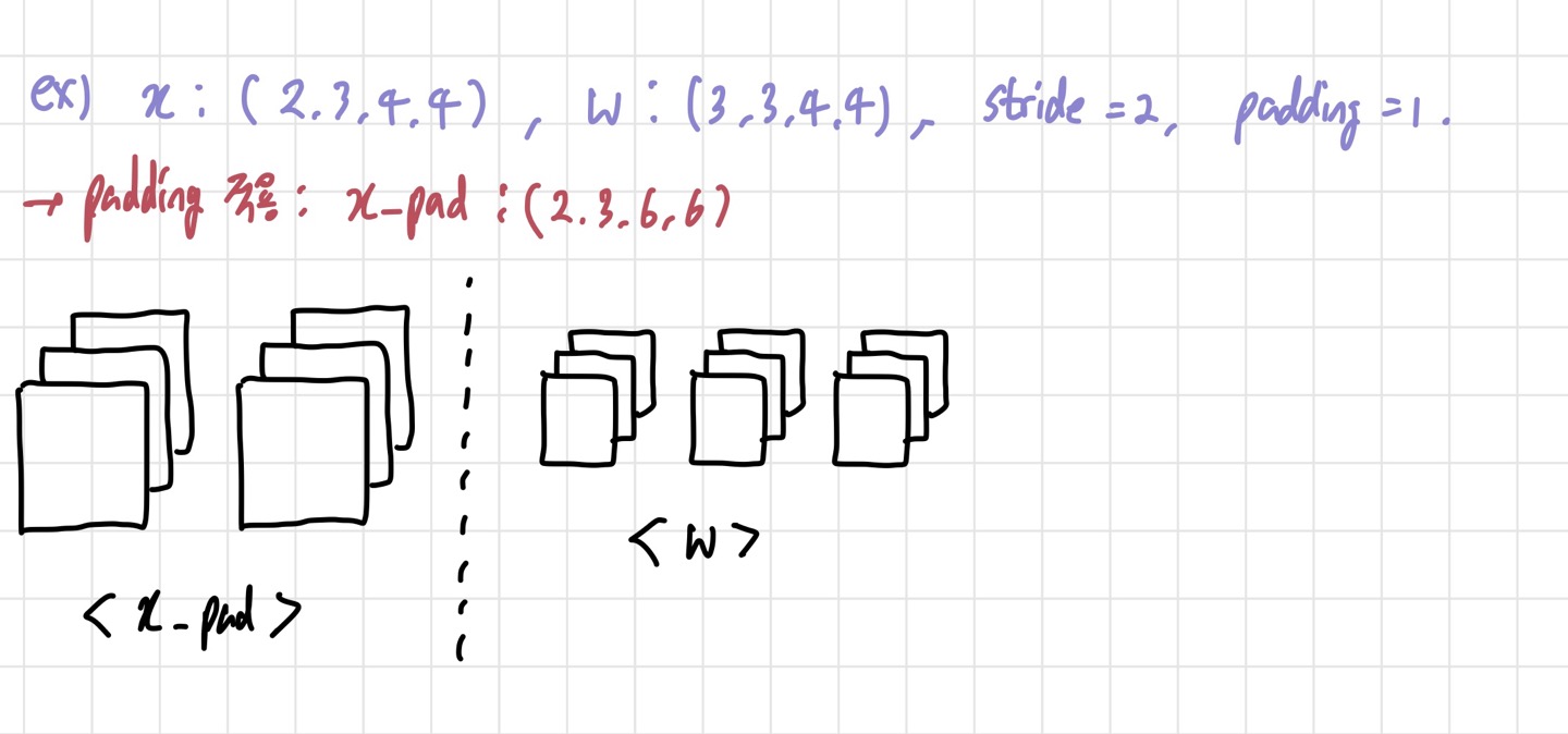
과제에서 주는 input과 filter shape을 가지고 생각해보자. input이 (2,3,4,4) 라는 것은 3개의 채널을 가진 4x4 크기의 input들이 2개 있다는 뜻이고, $W$가 (3,3,4,4)라는 뜻은 채널 3개짜리의 4x4 filter가 3개 사용되었다는 뜻이다. 여기서 주의할 점은 padding=1이기 때문에 input size가 변한다는 것이다. 변한 input size를 $x_{pad}$라고 표현하겠다.

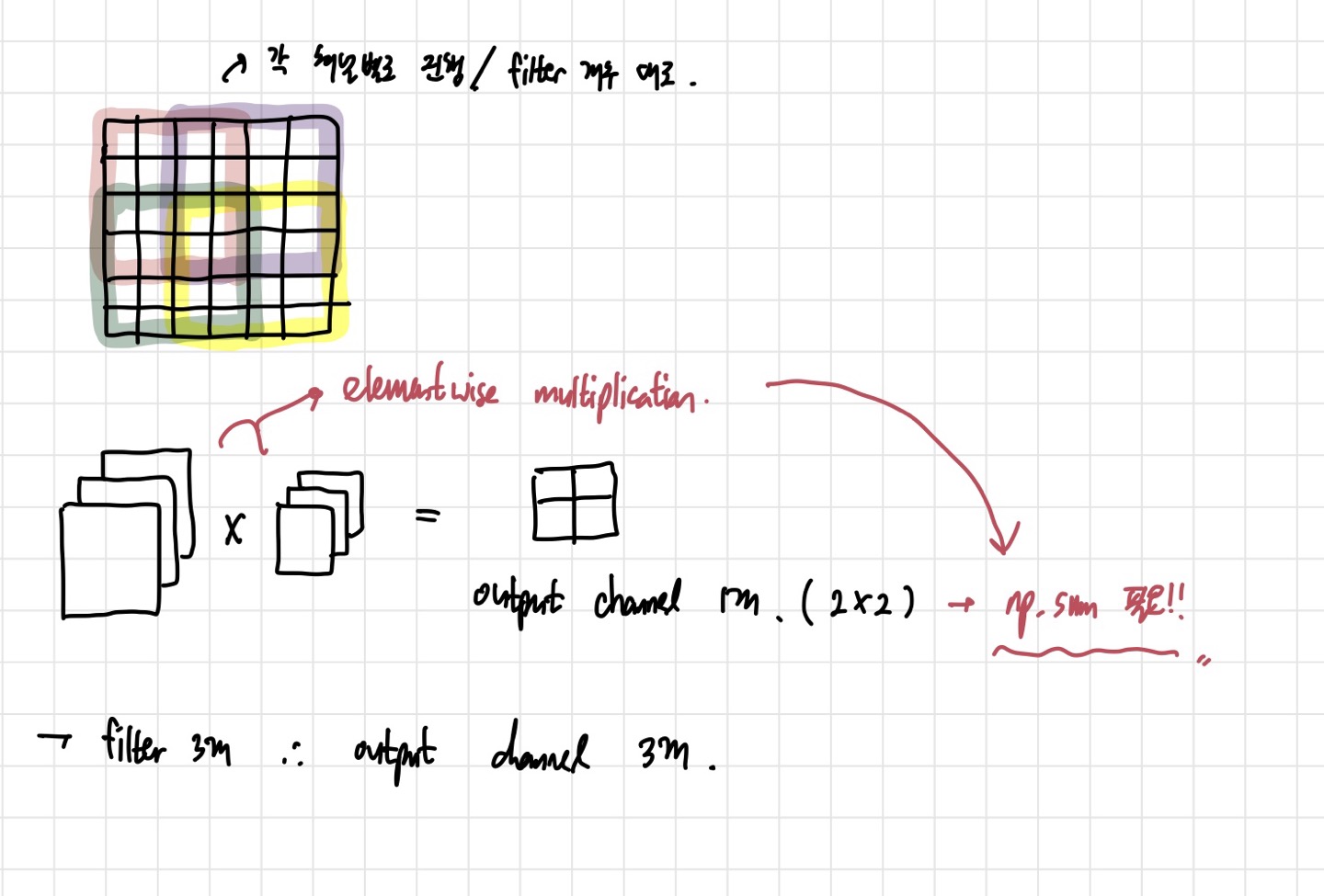
  기본적인 계산은 위의 사진처럼 진행된다. 6x6 크기의 사각형에 형광펜이 칠해진 부분은 각 input channel에서 filter가 어떻게 곱해져서 output pixel이 나오게 되는지에 대한 그림이다. 중요한 것은 그 아래에 있는 elementwise multiplication이다. 하나의 input과 하나의 filter를 계산하면, 채널이 3개가 된다. 그러나 output을 표현할 때 filter 1개당 하나의 output channel을 가져야 하므로, np.sum을 해주어야 한다. 이 결과 2x2 크기의 output channel 한 개를 갖게 된다.
 나는 간단하게 이해하기 위해 이 정도만 그렸지만, 이해가 안된다면 위의 사진과 같은 방식으로 계속 그려서 이해할 수 있다. 그리고 이렇게 이해하고 나면, conv_forward_naive 함수도 차원만 신경쓰면 무리없이 구현할 수 있다.

2. conv_backward_naive

def conv_backward_naive(dout, cache):
    ###########################################################################
    # TODO: Implement the convolutional backward pass.                        #
    ###########################################################################
    # *****START OF YOUR CODE (DO NOT DELETE/MODIFY THIS LINE)*****
    x, w, b, conv_param = cache
    stride=conv_param['stride']
    pad=conv_param['pad']
    N=x.shape[0]
    F=w.shape[0]
    H=x.shape[2]
    W=x.shape[3]
    HH=w.shape[2]
    WW=w.shape[3]
    H_out= 1+ (H+2*pad-HH)//stride
    W_out= 1+ (W+2*pad-WW)//stride
    pad_width=[(0,0),(0,0),(pad,pad),(pad,pad)]
    x_pad= np.pad(x,pad_width,mode='constant')
    dw = np.zeros_like(w)
    dx = np.zeros_like(x_pad)
    db = np.zeros_like(b)
    for i in range(N): #iterate for N inputs.
      for j in range(F): # number fo filters
        for p in range(H_out):
          for q in range(W_out):
             H_now=p*stride
             W_now=q*stride
             db[j]+=dout[i,j,p,q]
             dw[j]+=dout[i,j,p,q]*x_pad[i,:,H_now:H_now+HH,W_now:W_now+WW]
             dx[i,:,H_now:H_now+HH,W_now:W_now+WW]+=dout[i,j,p,q]*w[j,:,:,:]

    dx=dx[:,:,pad:-pad,pad:-pad]# get rid of the padding. 
    # *****END OF YOUR CODE (DO NOT DELETE/MODIFY THIS LINE)*****
    ###########################################################################
    #                             END OF YOUR CODE                            #
    ###########################################################################
    return dx, dw, db

  이전에 구현했던 함수와 마찬가지로 $dx, dw, db$는 각각 $x,w,b$와 동일한 shape을 가진다. conv_forward를 구현했으면 backward를 구현하는 것은 그닥 어렵지 않다. 따지고 보면 CNN도 $y=wx+b$의 확장이므로, $dx=w*dout, dw=x*dout, db=dout$의 기본적인 결을 따라가면 된다. 다만 조심해야 할 것은 차원이다. 일단 우리가 padding을 통해 forward pass를 진행했으므로, 여기서도 padding을 한 다음에 gradient를 계산한다. $dx$에 대해서만 마지막에 padding된 부분들을 없애고 원래 $x$의 shape으로 만들어주면 된다. (코드의 맨 마지막 줄에 해당한다.)
  과제에서는 $x$: (4,3,5,5), $w$: (2,3,3,3), stride=1, padding=1, dout=(4,2,5,5) 의 크기들을 줬다. 이를 토대로 우리는 $dx,dw,db$를 계산하면 되는 것이다. 먼저, db=dout을 따른다. 그러나 하나의 filter는 하나의 output channel을 책임지므로, db[j]+=dout[i,j,p,q]를 해주면 된다. 쉽게 말하면 dout의 모든 픽셀들의 합을 더해준다는 뜻이다. 비슷한 논리로 $dw$도 filter별로 backprop을 진행해주어야 한다. filter가 forward pass 때 지나간 경로를 그대로 따라가면서 거기에 dout만 곱해주면 된다. 마지막으로 dx는 각 input sample별로 계산해야 한다. dout에 w를 filter별로 곱해서 dx에 더해주면 된다.

3. ThreeLayerConvNet

class ThreeLayerConvNet(object):
    """
    A three-layer convolutional network with the following architecture:

    conv - relu - 2x2 max pool - affine - relu - affine - softmax

    The network operates on minibatches of data that have shape (N, C, H, W)
    consisting of N images, each with height H and width W and with C input
    channels.
    """

    def __init__(
        self,
        input_dim=(3, 32, 32),
        num_filters=32,
        filter_size=7,
        hidden_dim=100,
        num_classes=10,
        weight_scale=1e-3,
        reg=0.0,
        dtype=np.float32,
    ):
        
        self.params = {}
        self.reg = reg
        self.dtype = dtype

        ############################################################################
        # TODO: Initialize weights and biases for the three-layer convolutional    #
        # network. Weights should be initialized from a Gaussian centered at 0.0   #
        # with standard deviation equal to weight_scale; biases should be          #
        # initialized to zero. All weights and biases should be stored in the      #
        #  dictionary self.params. Store weights and biases for the convolutional  #
        # layer using the keys 'W1' and 'b1'; use keys 'W2' and 'b2' for the       #
        # weights and biases of the hidden affine layer, and keys 'W3' and 'b3'    #
        # for the weights and biases of the output affine layer.                   #
        #                                                                          #
        # IMPORTANT: For this assignment, you can assume that the padding          #
        # and stride of the first convolutional layer are chosen so that           #
        # **the width and height of the input are preserved**. Take a look at      #
        # the start of the loss() function to see how that happens.                #
        ############################################################################
        # *****START OF YOUR CODE (DO NOT DELETE/MODIFY THIS LINE)*****
        C=input_dim[0]
        H=input_dim[1]
        W=input_dim[2]

        self.params['W1']=np.random.randn(num_filters,C,filter_size,filter_size)*weight_scale
        self.params['b1']=np.zeros((num_filters,)) # parameters for conv layer

        self.params['W2']=np.random.randn(H*W*num_filters//4,hidden_dim)*weight_scale # divide by 4 due to 2*2 pooling 
        self.params['b2']=np.zeros((hidden_dim,))
        self.params['W3']=np.random.randn(hidden_dim,num_classes)*weight_scale
        self.params['b3']=np.zeros((num_classes,))

  이 부분은 정해진 architecture대로 three-layer net을 만들면 된다. Conv layer는 filter의 수가 output channel 수가 되기 때문에 이를 맞춰주어야 한다. 주의할 점은 Conv layer에서 FC layer로 넘어가는 부분인데, 2x2 pooling이 있기 때문에 4로 나누어주면 크기가 맞춰진다. 그 밖에 내용들은 fc_net.py에서 하던 것과 거의 유사하다.

4. spacial_batchnorm_forward

def spatial_batchnorm_forward(x, gamma, beta, bn_param):
    
    out, cache = None, None

    ###########################################################################
    # TODO: Implement the forward pass for spatial batch normalization.       #
    #                                                                         #
    # HINT: You can implement spatial batch normalization by calling the      #
    # vanilla version of batch normalization you implemented above.           #
    # Your implementation should be very short; ours is less than five lines. #
    ###########################################################################
    # *****START OF YOUR CODE (DO NOT DELETE/MODIFY THIS LINE)*****
    N,C,H,W=x.shape
    x=np.moveaxis(x,1,-1)# shape: (N,H,W,C)
    x=x.reshape(-1,C)# batch normalization per feature map(=each channel)
    out,cache=batchnorm_forward(x,gamma,beta,bn_param) 
    out=np.moveaxis(out.reshape(N,H,W,C),-1,1) #make the output the same shape as x. shape:(N,C,H,W)

    # *****END OF YOUR CODE (DO NOT DELETE/MODIFY THIS LINE)*****
    ###########################################################################
    #                             END OF YOUR CODE                            #
    ###########################################################################

    return out, cache

   Conv layer에서의 batchnorm을 구현하는 함수이다. Conv layer의 경우, FC layer와는 다르게 channel wise batch normalization을 진행한다. 내가 구현하면서 힘들었던 부분은 배열의 차원을 이동시키고, reshape하는 것이었다. 정확히는 언제 np.reshape를 사용하고 언제 np.moveaxis를 사용할지가 헷갈렸었다. 먼저 두 함수가 어떤 기능을 하는지부터 알아보자.

1) np.moveaxis(arr,a,b): 배열 arr에서 차원 a를 차원 b로 옮겨준다. 차원을 rearrange하는 것이지만, data는 보존한다.
ex) np.moveaxis(x,1,-1)은 x의 1번 차원을 마지막 차원으로 옮기라는 뜻이다. 만약 x의 shape이 (3,2,4) 였다면, 함수 적용 후 shape은 (3,4,2)가 되는 것이다.
2) np.reshape(x,(shape)): 배열을 지정한 shape에 맞게 변형시켜준다. 이전과는 다른 새로운 shape이고, 배열 원소들의 순서는 보존된다. (순서가 보존되는 것이지 차원별 크기는 변할 수 있다.)

  함수들이 이러한 기능을 가지고 있기 때문에, 위에서 spacial batchnorm을 구현할 때 moveaxis를 먼저 해주어 C를 마지막 차원으로 보낸 후 reshape를 진행한다. 만약 바로 reshape를 진행하면 차원 간의 정보가 뒤섞이게 되어 좋지 않다. spacial_batchnorm_backward도 이런 식으로 np.reshape와 np.moveaxis를 사용해 비교적 쉽게 구현할 수 있다.

5. Group Normalization

def spatial_groupnorm_forward(x, gamma, beta, G, gn_param):
    
    out, cache = None, None
    eps = gn_param.get("eps", 1e-5)
    ###########################################################################
    # TODO: Implement the forward pass for spatial group normalization.       #
    # This will be extremely similar to the layer norm implementation.        #
    # In particular, think about how you could transform the matrix so that   #
    # the bulk of the code is similar to both train-time batch normalization  #
    # and layer normalization!                                                #
    ###########################################################################
    # *****START OF YOUR CODE (DO NOT DELETE/MODIFY THIS LINE)*****
    N,C,H,W=x.shape
    xg=x.reshape([N,G,C//G,H,W])
    x_mean=np.mean(xg,axis=(2,3,4),keepdims=True)#(N,G,1,1,1)
    x_var=np.var(xg,axis=(2,3,4),keepdims=True)#(N,G,1,1,1)
    x_std=np.sqrt(x_var+eps)
    x_hat=(xg-x_mean)/x_std
    x_hat=x_hat.reshape([N,C,H,W])
    out=gamma*x_hat+beta
    cache = x, x_mean, x_var,x_std, gamma, x_hat, G

    # *****END OF YOUR CODE (DO NOT DELETE/MODIFY THIS LINE)*****
    ###########################################################################
    #                             END OF YOUR CODE                            #
    ###########################################################################
    return out, cache

  Groupnorm도 과제에 나와 있는 논문을 읽고 구현하면 된다. 다만, layer norm에서의 방식과 유사하게 구현하는데, 그때보다 차원이 많아져서 조금 복잡하다.

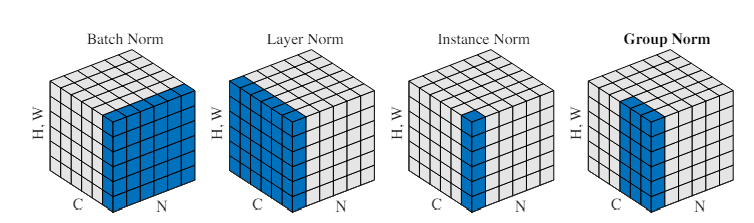
  기본적인 intuition은 이것이다. batchnorm의 batch size 의존도 문제를 해결하기 위해 여러 방법들이 그동안 제안되어 왔다. 그러나 문제가 완벽히 해결된 것은 아니었다. 때문에 저자는 batch size를 이용하지 않는 방안을 고안하고자 했다. 결론적으로 GN은 layer norm과 instance norm의 중간 형태를 가진다. 그룹을 만들어 여러 개의 채널들을 묶는 것이다. 만약 채널이 6개인데 그룹이 2개라면, 각 그룹당 3개의 채널을 갖게 되는 것이다. 이때 평균과 분산은 (H,W) axis와 C/G axis에 대해서 구한다.

def spatial_groupnorm_backward(dout, cache):
    
    dx, dgamma, dbeta = None, None, None

    ###########################################################################
    # TODO: Implement the backward pass for spatial group normalization.      #
    # This will be extremely similar to the layer norm implementation.        #
    ###########################################################################
    # *****START OF YOUR CODE (DO NOT DELETE/MODIFY THIS LINE)*****

    x, x_mean, x_var,x_std, gamma, x_hat, G=cache
    N,C,H,W=dout.shape
    xg=x.reshape([N,G,C//G,H,W])
    M=C//G*H*W
    dgamma=np.sum(dout*x_hat,axis=(0,2,3)).reshape(1,C,1,1)
    dbeta=np.sum(dout,axis=(0,2,3)).reshape(1,C,1,1)

    dvar=np.sum((dout*gamma).reshape(xg.shape)*(xg-x_mean)*(-0.5)*(x_std**(-3)),axis=(2,3,4),keepdims=True)
    du=np.sum(((-dout*gamma).reshape(xg.shape)/x_std),axis=(2,3,4),keepdims=True)+ dvar*np.sum((-2*(xg-x_mean)),axis=(2,3,4),keepdims=True)/M
    dx= (dout*gamma).reshape(xg.shape)/x_std +dvar*2*(xg-x_mean)/M + du/M
    dx=dx.reshape(N,C,H,W)
    # *****END OF YOUR CODE (DO NOT DELETE/MODIFY THIS LINE)*****
    ###########################################################################
    #                             END OF YOUR CODE                            #
    ###########################################################################
    return dx, dgamma, dbeta

  backward pass도 layer norm과 비슷하다. 차원이 어떻게 될 지에 대한 생각을 잘 해야 한다. 나의 경우는 dvar, du등 중간 값들의 shape이 어떤지를 자세히 봤던 것 같다.
 조금 더 자세히 들여다 보자. 위에서 x_mean과 x_var는 H,W,C/G 축에 대해서 구하는 것이라고 했다. group normalization을 위해 x의 shape을 (N,G,C//G,H,W)로 바꾸어 놓았기 때문에 mean과 variance의 shape은 (N,G,1,1,1)이 된다. 이를 이용해 x_hat을 구하고 다시 원래의 x shape인 (N,C,H,W)로 바꾸어 주면 된다. backward pass에서도 dvar와 du의 크기가 (N,G,1,1,1)이 되어야 하기 때문에 이에 맞춰 np.sum을 진행해주면 된다.

내 풀이 링크:

https://github.com/danlee0113/cs231n