나의 논문을 이해하고 정리하는 기준은 아래와 같다.

• 항목을 기준으로 정리하였다.
• 연구 목적, 목표와 모델 구성을 위한 아이디어와 구현을 중심으로 결과를 파악하는데 중점을 두었다.
• 결국에는 모델의 구성 아이디어에 따른 효과를 파악하는 것을 목적으로 논문을 정리한다. (논문간의 비교를 위한 자세한 서술을 분석하고 이해하지 않는다.)

Abstract

• 분류
  : classification
• 사용 기술
  : deep convolutional neural network
• 데이터
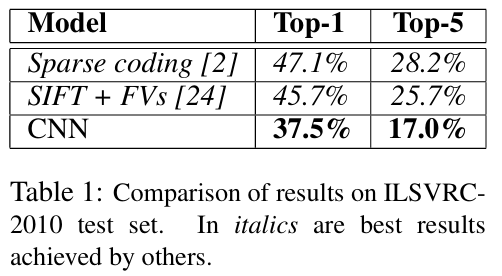
  : ImageNet LSVRC-2010 (the 1.2 million images, the 1000 different classes)
• 성능
  : top-1 and top-5 error rates of 37.5% and 17.0% (state-of-the-art)
• 비고
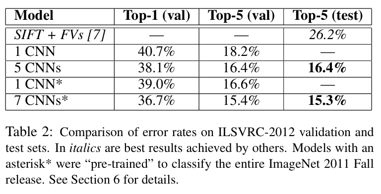
  : a variant of this model in the
  ILSVRC-2012 competition (a winning top-5 test error rate of 15.3%을 얻음, compared to 26.2% achieved by the second-best entry.)

'' 핵심은 deep convolutional neural network 모델을 사용하여 이미지 분류에서 뛰어난 성과를 얻었다는 것이다.''

모델 구현

3 The Architecture

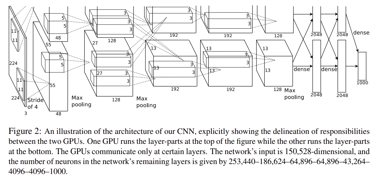
Figure 2에 모델을 요약한 그림이다. 전체 구성을 Figure2에서 보이는데로 적어보면, Input_layer →
CNN1 → Max pooling → CNN2 → Max pooling → CNN3 → CNN4 → CNN5 → Max pooling → Dense1 → Dense2 → Dense3 이다. Figure 2에서는 이 정도를 볼 수 있고, 다른 부분을 읽으면서 더 자세히 모델을 파악해보자.

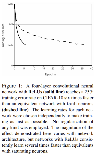
3.1 ReLU Nonlinearity

3.1에는 모델에 ReLU를 사용했다는 것이다. 아래 Figure 1에서 볼 수 있듯이 학습이 6배나 빠르다는 것을 볼 수 있다. ReLU는 4개의 CNN에 사용되었다.

3.3 Local Response Normalization

논문에서는 평가 데이터로 최적화한 변수는 k = 2, n = 5, α = 10−4, and β = 0.75 이고, ReLU 다음에 온다.

3.4 Overlapping Pooling

non-overlapping인 (2x2)-pooling, stride = 2일 때와 비교할 때 (3 x 3) pooling, stride = 2 일 때 the top-1 and top-5 error rates by 0.4% and 0.3%이 감소하였다.

3.5 Overall Architecture

앞 서 Figure 2에서 요약한, 5-convolutional와 3개 fullyconnected로 구성되어 있고 마지막 last fully-connected layer는 a 1000-way softmax가 있다. Response-normalization layers는 the first and second convolutional layers에 온다.
Max-pooling layers는 response-normalization layers와 5번째 convolutional layer에 온다. The ReLU는 모든 convolutional 바로 다음과 fully-connected layer에 온다.

(layers을 총리하면서 주의할점은 논문에서는 2 GPU 분산을 사용해서 총 kernels 수의 0.5배로 서술하였다. 그런데 자세히 보면 서술 오류로 총 kernels을 서술하기도 하였다.)

• input은 224x224x3 이미지다.
• C1-layer : 11x11x3, stride = 4, 96 kernels
• C2-layer : 5x5x48(이때 GPU로 분산이 되어 있어서, 1GPU에서는 96kernels로 진행해야한다), 256 kernels.
• C3-layer : 3x3x256, 384 kernels.(서술은 되지 않았지만 그림에서 보면 384 kernels이다.
• C4-layer : 3x3x192, 384 kernels. (1GPU에서는 filters가 384이다.)
• C5-layer : 3x3x192, 256 kernels. (1GPU에서는 filters가 384이다.)
• F1-layer : 4096 neurons
• F2-layer : 4096 neurons
• 1000-softmax layer

이제 모델을 코드로 구현해보자.
모델 코드

4 Reducing Overfitting

이 chapter는 Overfitting을 줄이기 위한 기법을 소개했다.
모델이 60 million parameters을 가지고 있는데 1000 classes of ILSVRC는 학습시키기에 충분하지 않은 데이터를 가지고 있다. 그래서 overfitting을 고려해야하는데 아래는 overfitting을 줄이는 두 가지의 방법을 서술하였다.

4.1 Data Augmentation

1) 256 x 256 images로 부터 random 224 x 224 patches을 추출(그리고 horizontal reflections을 한다.)한 것으로 학습시킨다. (Figure2에서 224x224x3인 이유.)
2) 학습 데이터의 RGB 채널의 intensities을 대체한다. (PCA을 수행) : top-1 error rate by over 1%의 효과.

4.2 Dropout

첫 번째와 두 번째 fully-connected layers에 사용.

5 Details of learning

stochastic gradient descent (momentum of 0.9, and
weight decay of 0.0005)로 batch size를 128로 하여 진행하였다.

• 각 layer의 가중치 초기화는 a zero-mean Gaussian distribution with standard deviation 0.01로 하였다.

• 편향(biases)의 초기화는 the second, fourth, and fifth convolutional layers, as well as in the fully-connected hidden layers, with the constant 1이다.

• We initialized the neuron
  biases in the remaining layers with the constant 0.

• The heuristic which we followed was to divide the learning rate by 10 when the validation error
  rate stopped improving with the current learning rate.

• The learning rate was initialized at 0.01 and reduced three times prior to termination.

• We trained the network for roughly 90 cycles through the
  training set of 1.2 million images, which took five to six days on two NVIDIA GTX 580 3GB GPUs.

  6 Results