VERY DEEP CONVOLUTIONAL NETWORKS FOR LARGE-SCALE IMAGE RECOGNITION

논문 원본

ABSTRACT

• convolutional network을 깊게(depth)함.
• (3×3) convolution filters를 가지는 architecture을 사용해서 깊이를 증가시키며 평가하였는데 16에서 19층으로 깊이의 모델에서 상당한 향상을 보임.
• ImageNet Challenge 2014의 기본이 됨.
• 지역화(localisation)에서 1위, classification tracks에서 2위를 함.
• 다른 datasets에서도 일반화 된다는 것을 보임 (SOTA).
• 대중적으로 이용할 수 있도록 두 개의 가장 성능이 좋은 ConvNet 만듬.

2 CONVNET CONFIGURATIONS

2.1 ARCHITECTURE

• a fixed-size 224 × 224 RGB image.
• RGB 평균 값을 빼준 전처리만 함.
• a stack of 3 × 3 convolutional (conv.) layers을 사용
• 구성 중간에는 1 × 1 convolution filters도 사용했는데 input channels 을 a linear transformations하는 기능을 한다 (followed by non-linearity).
• The convolution stride is fixed to 1 pixel; the spatial padding of conv.
• Spatial pooling은 다섯개의 max-pooling layers (2 × 2 pixel window, with stride 2.)를 사용함.
• (공통) A stack of convolutional layers 다음에 three Fully-Connected (FC) layers가 온다 ( 4096 channels 2개, 1000way ILSVRC classification 1개, 맨 마지막에 soft-max layer.
• 모든 hidden layers 에는 ReLU가 온다.

2.2 CONFIGURATIONS

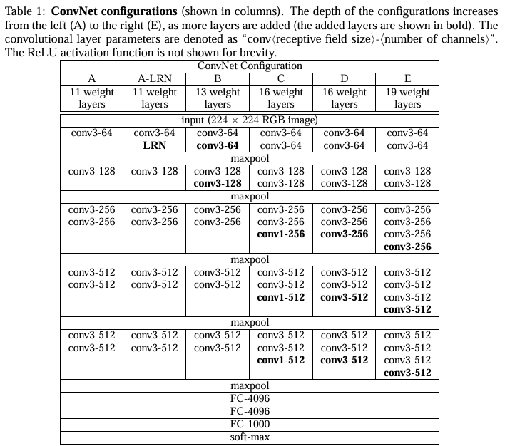
• 구성들은 Table 1에서 보여주는데 열들(A-E)이 모델들을 보여준다.
• 오직 차이점은 깊이인데, 11 layer인 A (8c conv. 와 3 FC layers) 부터 19 layers 인 E (16 conv.와 3 FC layers) 임을 보여준다.

3 CLASSIFICATION FRAMEWORK

training and evaluation에 대한 서술한 장.

3.1 TRAINING

• The batch size was set to 256, momentum to 0.9.
• The training was regularised by weight decay (the L2 penalty multiplier set to
  5·10−4) and dropoutregularisation for the first two fully-connected layers (dropout ratio set to 0.5).
  The learning rate was initially set to 10−2, and then decreased by a factor of 10 when the validation
  set accuracy stopped improving. In total, the learning rate was decreased 3 times, and the learning
  was stopped after 370K iterations (74 epochs).
• we initialised the first four convolutionallayers and the last three fully
  connected layers with the layers of net A (the intermediatelayers were initialised randomly).
• For random initialisation (where applicable), we sampled the weights from a normal distribution
  with the zero mean and 10−2 variance. The biases were initialised with zero.
• Toobtain the fixed-size224×224ConvNetinputimages,they wererandomlycroppedfromrescaled
  training images (one crop per image per SGD iteration).
• To further augment the training set, the
  crops underwentrandomhorizontal flipping and randomRGB colourshift .
• Training image rescaling is explained below.

Training image size.

• approach 1 : S = 256 and S = 384을 사용함.
  - 먼저 S = 256로 학습 한 후에, S = 256으로 학습된 weights를 가지고 S = 384를 학습 시킴 (initial learning rate of 10−3).
• approach 2 : multi-scale training. 임의의 샘플 S의 각 학습 이미지를 개별적으로 rescaled함 (from a certain range [Smin,Smax] (we used Smin = 256 and Smax = 512)).
• pre-trained with fixed S = 384로 fine-tuning all layers of a single-scale model.

3.2 TESTING

3.3 IMPLEMENTATION DETAILS

On a system equipped with four NVIDIATitan Black GPUs, traininga single net took 2–3weeks dependingonthe architecture.