논문 : https://arxiv.org/pdf/1311.2524

Abstract

• 지난 수년 동안 canonical PASCAL VOC dataset로 측정된 객체 탐지 성능은 정체되었음.
• 가장 성능이 좋은 방법은 전형적으로 다수의 낮은 레벨의 이미지 특성들과 높은 레벨의 context와 함께 전형적으로 결합하는 복잡한 앙상블 시스템임.
• 이 논문에서는, mean average precision(mAP)가 향상된 단순하고 확장 가능한 탐지 알고리즘을 제안함.
• 접근 방법
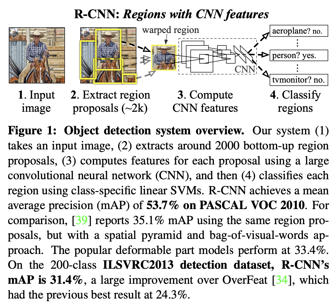
  (1) CNNs을 localize(현지화)와 segment objects을 위해 bottom-up region proposals에 적용함.
  (2) 라벨된 training data가 부족할 때, 도메인에 특화된 미세조정(fine-tuning)에 의해 따라오는 보조 작업을 위해 사전-학습을 지도는 상당한 성능 향상을 가져옴.
• CNNs와 지원 제안을 결합하므로, 이 방법을 R-CNN이라 부름 (Regions with CNN features).
• OverFeat(CNN과 비슷한 구조 기반으로 sliding-window detector를 제안한 모들)과 비교함.
• R-CNN은 200-class ILSVRC2013 detection에서 큰 차이로 OverFeat의 성능이 좋음을 찾음.

Figures and Tables

Introduction

• CNN 분류 결과(ImageNet을 활용)가 PASCAL VOC Challenge의 객체 탐지(object detection)결과에 얼마나 일반화할 수 있는지에 대한 의문임.

• 이미지 분류와 객체 탐지 사이의 차이를 연결하여 문제를 대답함.
  1. 깊은 신경망으로 객체를 지역화함.

  2. 주석화된 작은 양의 탐지 테이터를 high-capacity model로 훈련시킴.

• 두 번째 도전과제는 큰 CNN을 학습 시킬 충분히 이용할 라벨된 데이터의 부족임. 이 문제의 편리한 해결은 unsupervised pre-training을 사용하는 것임.

• 큰 보조 데이터(ILSVRC)의 사전 학습을 작은 데이터셋 (PASCAL)에 fine-tuning을 함.

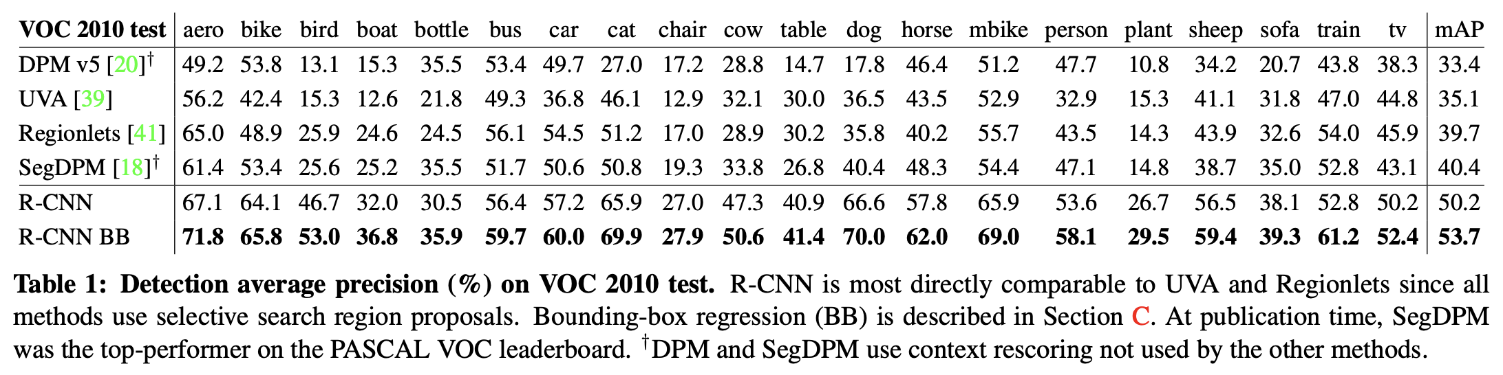
• fine-tuning 이후, VOC 2010에서 mAP 54%로 HOG 기반 deformable part model(DPM)의 33% mAP를 비교하면 성능이 향상됨

Conclusions

• PASCAL VOC 2012의 이전 결과 보다 상대적으로 30%나 향상시킴.
• Insights:
  1. high-capacity convolutional neural networks를 지역화와 segment objects를 위해 bottom-up region proposals에 적용함.
  2. 라벨된 학습 데이터가 부족할 때 학습시킨 CNNs를 활용하는 것임 (다양한 부족한 학습 데이터를 가진 컴퓨터 비전 문제에 효과적일 것으로 추정함).
• 컴퓨터 비전의 고전적인 도구와 딥러닝(bottom-up region proposals과 CNN)을 결합하여 사용하여 결과를 얻음.

2. Object detection with R-CNN

3개의 모듈로 구성됨
1. category-independent region proposals.
(These proposals define the set of candidate detections available to our detector.)
2. a large CNN (각 region에서 a fixed-length feature vector를 추출)
3. 고전적 특별한 linear SVMs의 집합(set).

2.1. Module design

Region proposals.
Feature extraction.
We extract a 4096-dimensional fea- ture vector from each region proposal using the Caffe [24] implementation of the CNN described by Krizhevsky et al. [25]. Features are computed by forward propagating a mean-subtracted 227 × 227 RGB image through five con- volutional layers and two fully connected layers. We refer readers to [24, 25] for more network architecture details.
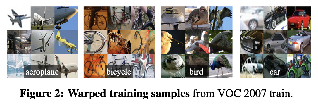
Regardless of the size or aspect ratio of the candidate region, we warp all pixels in a tight bounding box around it to the required size.
Prior to warping, we dilate the tight bounding box so that at the warped size there are ex- actly p pixels of warped image context around the original box (we use p = 16). Figure 2 shows a random sampling of warped training regions.

2.3. Training
Supervised pre-training.
We discriminatively pre-trained the CNN on a large auxiliary dataset (ILSVRC2012 clas- sification) using image-level annotations only (bounding- box labels are not available for this data).

Domain-specific fine-tuning.
we continue stochastic gradient descent (SGD) training of the CNN parameters using only warped region proposals.
For VOC, N = 20 and for ILSVRC2013, N = 200. We treat all region proposals with ≥ 0.5 IoU overlap with a ground-truth box as positives for that box’s class and the rest as negatives.
We start SGD at a learning rate of 0.001 (1/10th of the initial pre-training rate), which allows fine-tuning to make progress while not clobbering the initialization.
In each SGD iteration, we uni- formly sample 32 positive windows (over all classes) and 96 background windows to construct a mini-batch of size 128.

Object category classifiers.
3.1. Visualizing learned features
The pool5 feature map is 6 × 6 × 256 = 9216- dimensional.
Ignoring boundary effects, each pool5 unit has a receptive field of 195×195 pixels in the original 227×227 pixel input.
3.2. Ablation studies
3.3. Network architectures
The network has a homogeneous structure consisting of 13 layers of 3 × 3 convolution kernels, with five max pooling layers interspersed, and topped with three fully-connected layers.
We refer to this network as “O-Net” for OxfordNet and the baseline as “T-Net” for TorontoNet.
To use O-Net in R-CNN, we downloaded the pub- licly available pre-trained network weights for the VGG ILSVRC 16 layers model from the Caffe Model Zoo.1 We then fine-tuned the network using the same pro- tocol as we used for T-Net. The only difference was to use smaller minibatches (24 examples) as required in order to fit within GPU memory.
The results in Table 3 show that R- CNN with O-Net substantially outperforms R-CNN with T- Net, increasing mAP from 58.5% to 66.0%.
However there is a considerable drawback in terms of compute time, with the forward pass of O-Net taking roughly 7 times longer than T-Net.
4.2. Region proposals
We followed the same region proposal approach that was used for detection on PASCAL.
4.3. Training data
Training data is required for three procedures in R-CNN: (1) CNN fine-tuning, (2) detector SVM training, and (3) bounding-box regressor training.
5. Semantic segmentation
CNN features for segmentation.
all of which begin by warping the rectangular window around the re- gion to 227 × 227.