Divide and Conquer

• Divide the problem into a nnumber of subproblems
• Conquer the subproblems by solving them recursively. If the subproblem sizes are small enough, just solve them in a straightforward manner.
• Combine the solutions to the subproblems into the solution for the original problem.

Key Observations

1. The problem can be split into subproblems.
2. The optimal solution can be defined in terms of optimal subproblems.

Conditions for DP

1. Simple subproblems : The subproblems can be defined in terms of a few variables.
2. Subproblem optimality : The global optimum value can be defined in terms of optimal subproblems
3. Subproblem overlap : The subproblems are not independent, but instead they overlap (hence, should be constructed bottom-up)

Matrix Chain Multiplication

Brute-Force Approach

ex) B : 3x100 / C : 100 x 5 / D : 5 x 5
(BC)D = (3 x 100 x 5) + (3 x 5 x 5) = 1500 + 75 = 1575
B(CD) = (100 x 5 x 5) + (3 x 100 x 5) = 2500 + 1500 = 4000

• 계산 순서에 따라 연산 횟수가 달라진다.
• 따라서 각 연산 횟수들을 구한 후, 최선의 경우를 선택한다.

Running time

• 괄호를 치는 경우의 수가 n nodes로 구성된 binary tree의 수와 같다.
• 이는 지수이므로 매우 오래걸리는 알고리즘.

Greedy Algorithm

• Choose the local optimal iteratively
• Repeatedly select the product that uses the fewest operations
  ex) Computation of ABCD
  A : 10 x 5 / B : 5 x 10 / C : 10 x 5 / D : 5 x 10
  AB : 10 x 5 x 10 / BC : 5 x 10 x 5 / CD : 10 x 5 x 10
  -> BC 선택.
  A((BC)D) : 250 + 250 + 500 = 1000 ops

DP Approach

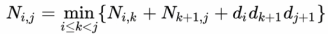
N_i, k와 N_k+1,j는 각 Subtree의 cost들을 의미하며, d_i, d_k+1, d_j+1은 이 subtree들을 곱하는 연산의 cost를 의미한다.

• N_[i,i+k], i <= k < j : i부터 k까지 원소들간의 연산의 최적해.
• Ai : d_i x d[i+1] 행렬.

Total Time Complexity is O(n^3)

Algorithm matrixChain(S):
	Input : sequence S of n matrices to be multiplied.
    Output : number of operations in an optimal paranethization of S
    
    for i <- 0 to n-1 do
    	N_i,i <- 0
    for b <- 1 to n-1 do
    	for i <- 0 to n-b-1 do
        	j <- i+b
            N_i,i <- +inf
            for k <- i to j-1 do
            	N_i,j <- min{N_i,j, N_i,k + N_k+1,j + d_i*d_k+1*d_j+1}

0-1 Knapsach Problem

Algorithm Knapsack(W, w, b)
	Input : Maximum weight W, weights w_i, and benefits b_i (i=0, ..., n).
    Output : B[i, j] (i=0,...,n, j=0,...,W) of the optimal knapsack solution.
    for w <- 0 to W do
    	B[0, w] <- 0		// DP Table Initialization
    for i <- 0 to n do
    	B[i, 0] <- 0		// DP Table Initialization
    for i <- i to n do
    	for w <- 0 to W do
        	if W_i <= w
            	if b_i + B[i-1, w-w_i] > B[i-1,w]
                	B[i,w] = b_i + B[i-1, w-w_i]
                else
                	B[i,w] = B[i-1,w]
             else
             	B[i,w] <- B[i-1, w]
	return B

Time complexity : O(nW)

Finding items in the Knapsack

• Backtracking
• Start from B[n, W], which is the maximal value of items in the Knapsack.

i <- n
k <- W
while i > 0 & k > 0
	if B[i,k] != B[i-1,k]
    	Mark the i-th item as in the knapsack
        i <- i-1
        k <- k-w_i
    else
    	i <- i-1		// Assume the i-th item is NOT in the knapsack

---

Analysis of 0-1 Knapsack Problem

Correctness of the algorithm

• 알고리즘은 모든 가능한 무게 용량에 대해 부분 최적해를 찾는다.
• knapsack으로 새 아이템을 넣을 때, knapsack 안에 어떤 아이템들이 있는지 모른 채로 새 아이템이 들어갈 공간을 만든다.
• 실제로 주어진 용량에 대해 모든 가능한 아이템들의 조합을 고려한 것.
• 삽입 순서는 시간 복잡도 분석과 연관이 없다.

Total running time

• Proportional to table size : O(Wn)
• Can be slow by setting the total capacity to an arbitrary large number.