[논문 리뷰] Neural Machine Translation by Jointly Learning to Align and Translate(바다나우 어텐션)

성율·2025년 3월 2일

Bahdanau Attention 논문 리뷰 및 구현

안녕하세요, 오늘은 Attention을 최초로 고안한 바다나우 어텐션 논문을 리뷰해보겠습니다.
논문에 나온 모델 아키텍처의 수식을 이해하고, numpy로 구현해보면서 모델의 이해도를 높여보겠습니다.

1. 소개

1.1 기존 Sequence-to-Sequence 모델의 한계

기존의 Sequence-to-Sequence(seq2seq) 모델은 입력 문장 전체를 하나의 고정된 크기의 벡터로 압축한 후, 이를 기반으로 번역문을 생성하는 방식을 사용했습니다. 이러한 접근 방식에는 크게 두 가지 한계가 있었습니다.

정보 손실: 긴 문장의 경우, 전체 정보를 하나의 고정된 크기의 벡터로 압축하는 과정에서 중요한 정보가 손실될 수 있습니다.
병목 현상: 문장이 길어질수록 더 많은 정보를 제한된 크기의 벡터에 저장해야 하므로, 성능이 급격히 저하되는 현상이 발생합니다.

예를 들어, "나는 어제 친구와 함께 맛있는 저녁을 먹었다"라는 문장을 번역할 때, 기존 seq2seq 모델은 이 모든 정보를 하나의 고정된 크기의 벡터에 담아야 했습니다. 이는 마치 A4 용지에 쓰여진 긴 문장을 포스트잇 크기로 압축하는 것과 비슷합니다.

1.2 Attention 메커니즘의 필요성

이러한 한계를 극복하기 위해 인간의 번역 과정을 참고했습니다. 실제로 사람은 긴 문장을 번역할 때, 전체 문장을 한 번에 기억했다가 번역하지 않습니다.

대신, 다음과 같은 과정을 거칩니다:
1. 선택적 집중: 현재 번역하려는 부분에 집중
2. 문맥 참조: 필요할 때마다 원문을 다시 확인
3. 점진적 번역: 부분적으로 나누어 번역을 수행

예를 들어, "나는 어제 친구와 함께 맛있는 저녁을 먹었다"를 영어로 번역할 때:
1. "나는" → "I"
2. "어제" → "yesterday"
3. "친구와 함께" → "with my friend"
식으로 진행하며, 각 단계에서 필요한 문맥을 참조합니다.

1.3 논문의 핵심 아이디어

이 논문에서는 다음과 같은 혁신적인 아이디어를 제시합니다:

동적인 Context 벡터
- 각 디코딩 단계마다 새로운 context 벡터 생성
- 현재 번역 중인 단어와 관련된 입력 부분에 집중
- 고정된 크기의 벡터 사용으로 인한 정보 손실 방지
Alignment 모델
- 입력 문장과 출력 문장 간의 단어 정렬 자동 학습
- 신경망 기반의 soft alignment 사용
- end-to-end 학습 가능한 구조
Bidirectional RNN
- 입력 문장의 양방향 문맥 고려
- 순방향, 역방향 정보를 모두 활용
- 더 풍부한 문맥 정보 포착

이러한 접근 방식의 장점:

문장 길이에 관계없이 일관된 성능
자연스러운 단어 정렬 생성
장거리 의존성 문제 해결

2. 모델 아키텍처

2.1 인코더 (Bidirectional RNN)

인코더는 입력 문장의 각 단어를 양방향으로 처리하는 Bidirectional RNN으로 구성됩니다.

인코더 동작 원리

입력 처리
- 각 단어 $x_t$ 를 임베딩 벡터로 변환
- 순방향, 역방향 GRU에 각각 입력
양방향 처리
- 순방향 GRU: 문장을 처음부터 끝까지 처리
- 역방향 GRU: 문장을 끝에서 처음까지 처리
상태 결합
- 각 위치에서 순방향, 역방향 상태를 결합
- 결합된 상태가 해당 위치의 최종 표현

인코더 수식

입력 시퀀스 $x = (x_1, \cdots, x_T)$ 에 대해:

순방향 GRU:

z_t^f = \sigma(W_z^f x_t + U_z^f h_{t-1}^f + b_z^f)\\ r_t^f = \sigma(W_r^f x_t + U_r^f h_{t-1}^f + b_r^f)\\ \tilde{h}_t^f = \tanh(W_h^f x_t + U_h^f(r_t^f \odot h_{t-1}^f) + b_h^f)\\ h_t^f = (1-z_t^f) \odot h_{t-1}^f + z_t^f \odot \tilde{h}_t^f\\

역방향 GRU도 동일한 구조로 계산됩니다.

최종 인코더 출력:
$h_t = [h_t^f; h_t^b]$

여기서 [;]는 벡터 연결(concatenation)을 의미합니다.

2.2 디코더

디코더는 각 시점에서 어텐션 메커니즘을 통해 입력 시퀀스의 특정 부분에 집중하며 번역을 생성합니다. 기존 seq2seq와 달리, 디코더는 매 시점마다 다음과 같은 과정을 거칩니다:

어텐션 계산
- 현재 디코더 상태와 모든 인코더 출력 간의 연관성 계산
- 연관성 점수를 기반으로 어텐션 가중치 생성
- 가중치를 사용해 context 벡터 생성
상태 업데이트
- context 벡터와 이전 출력을 결합하여 새로운 상태 생성
- GRU를 통한 상태 업데이트
- Teacher forcing을 통한 학습 안정화
출력 생성
- 업데이트된 상태를 사용하여 다음 단어 예측
- softmax를 통한 확률 분포 계산

디코더 수식

시점 t에서의 디코더 동작은 다음 수식들로 표현됩니다:

Context 벡터 계산:
$e_{tj} = v_a^T \tanh(W_a s_{t-1} + U_a h_j) \\ \alpha_{tj} = \frac{\exp(e_{tj})}{\sum_{k=1}^{T_x} \exp(e_{tk})} \\ c_t = \sum_{j=1}^{T_x} \alpha_{tj} h_j$
GRU 상태 업데이트:
$s_t = \text{GRU}([y_{t-1}, c_t], s_{t-1})\\ = (1-z_t) \odot s_{t-1} + z_t \odot \tilde{s}_t$
출력 생성:
$P(y_t|y_{<t}, x) = \text{softmax}(W_o[s_t, c_t] + b_o)$

여기서:

$s_t$ : 디코더의 현재 은닉 상태
$c_t$ : 현재 시점의 context 벡터
$y_{t-1}$ : 이전 시점의 출력
$h_j$ : j번째 인코더 은닉 상태
$\alpha_{tj}$ : t 시점에서 j번째 입력에 대한 어텐션 가중치

2.3 어텐션 메커니즘

어텐션 메커니즘은 디코더가 입력 시퀀스의 어느 부분에 집중할지 결정하는 핵심 컴포넌트입니다. 이는 다음 세 단계로 구성됩니다:

스코어 계산 (Alignment Model)
- 디코더의 현재 상태와 각 인코더 출력 간의 연관성 측정
- 가중치 행렬과 비선형 함수를 통한 변환
- 에너지 함수를 통한 스코어 도출
가중치 생성 (Softmax)
- 스코어를 확률 분포로 변환
- 소프트맥스 함수를 통한 정규화
- 모든 가중치의 합이 1이 되도록 보장
Context 벡터 생성 (Weighted Sum)
- 가중치와 인코더 출력의 가중합 계산
- 현재 시점에서 중요한 정보 추출
- 디코더의 다음 단어 예측에 활용

어텐션 수식 상세 설명

Alignment Score:
$e_{ij} = v_a^T \tanh(W_a s_{i-1} + U_a h_j)$

이 수식에서:

$v_a$ : 학습 가능한 벡터
$W_a, U_a$ : 학습 가능한 가중치 행렬
$s_{i-1}$ : 디코더의 이전 은닉 상태
$h_j$ : j번째 인코더 은닉 상태

Attention Weights:
$\alpha_{ij} = \frac{\exp(e_{ij})}{\sum_{k=1}^{T_x} \exp(e_{ik})}$
Context Vector:
$c_i = \sum_{j=1}^{T_x} \alpha_{ij}h_j$

이러한 방식으로, 모델은 입력 시퀀스의 모든 부분을 고려하면서도, 현재 번역에 가장 관련있는 부분에 더 높은 가중치를 부여할 수 있습니다.

3. 모델 구현

3.1 기본 구성요소

먼저 모델의 기본이 되는 GRU 셀을 구현해보겠습니다.

GRU 셀 구현

class GRUCell:
    def __init__(self, input_dim, hidden_dim):
        # 가중치 초기화
        self.Wz = np.random.randn(hidden_dim, input_dim) * 0.001
        self.Uz = np.random.randn(hidden_dim, hidden_dim) * 0.001
        self.bz = np.zeros((hidden_dim, 1))
        
        self.Wr = np.random.randn(hidden_dim, input_dim) * 0.001
        self.Ur = np.random.randn(hidden_dim, hidden_dim) * 0.001
        self.br = np.zeros((hidden_dim, 1))
        
        self.Wh = np.random.randn(hidden_dim, input_dim) * 0.001
        self.Uh = np.random.randn(hidden_dim, hidden_dim) * 0.001
        self.bh = np.zeros((hidden_dim, 1))
    
    def forward(self, x, h_prev):
        # GRU 셀의 순전파
        z = sigmoid(np.dot(self.Wz, x) + np.dot(self.Uz, h_prev) + self.bz)
        r = sigmoid(np.dot(self.Wr, x) + np.dot(self.Ur, h_prev) + self.br)
        h_tilde = np.tanh(np.dot(self.Wh, x) + np.dot(self.Uh, (r * h_prev)) + self.bh)
        h = (1 - z) * h_prev + z * h_tilde
        return h

활성화 함수 구현

def sigmoid(x):
    return 1 / (1 + np.exp(-x))

def softmax(x):
    exp_x = np.exp(x - np.max(x))
    return exp_x / exp_x.sum()

def tanh(x):
    return np.tanh(x)

3.2 전체 모델 구현

이제 앞서 구현한 컴포넌트들을 조합하여 전체 모델을 구현해보겠습니다.

class BahdanauNMT:
    def __init__(self, input_vocab_size, output_vocab_size, hidden_dim):
        self.hidden_dim = hidden_dim
        self.encoder = BidirectionalEncoder(input_vocab_size, hidden_dim)
        self.decoder = AttentionDecoder(hidden_dim, output_vocab_size)
        self.attention = BahdanauAttention(hidden_dim)
        
    def forward(self, x, y, teacher_forcing=True):
        # 인코딩
        encoder_states = self.encoder.forward(x)
        
        # 디코딩 초기화
        batch_size = len(x)
        max_len = len(y)
        decoder_state = np.zeros((batch_size, self.hidden_dim))
        
        outputs = []
        attentions = []
        
        # 디코딩
        for t in range(max_len):
            if t == 0:
                decoder_input = np.zeros((batch_size, self.output_dim))
            elif teacher_forcing:
                decoder_input = y[t-1]
            else:
                decoder_input = outputs[-1]
            
            # 어텐션 및 디코딩
            context, attention = self.attention.compute_attention(
                encoder_states, decoder_state)
            decoder_state = self.decoder.forward(
                context, decoder_input, decoder_state)
            
            # 출력 저장
            outputs.append(decoder_state)
            attentions.append(attention)
        
        return np.array(outputs), np.array(attentions)

4. 학습 및 추론

4.1 손실 함수 정의

모델의 학습을 위해 크로스 엔트로피 손실 함수를 사용합니다.

def cross_entropy_loss(predictions, targets):
    """
    predictions: (batch_size, vocab_size) - 소프트맥스 이전의 로짓값
    targets: (batch_size,) - 정답 인덱스
    """
    batch_size = len(targets)
    
    # 소프트맥스 적용
    probs = softmax(predictions)
    
    # 각 샘플의 손실 계산
    correct_logprobs = -np.log(probs[range(batch_size), targets])
    
    # 배치의 평균 손실 반환
    return np.mean(correct_logprobs)

4.2 최적화 방법

모델 학습을 위해 Adam 최적화 알고리즘을 구현합니다.

class Adam:
    def __init__(self, params, learning_rate=0.001, beta1=0.9, beta2=0.999, epsilon=1e-8):
        self.params = params
        self.lr = learning_rate
        self.beta1 = beta1
        self.beta2 = beta2
        self.epsilon = epsilon
        
        # 모멘텀 초기화
        self.m = {p: np.zeros_like(v) for p, v in params.items()}
        self.v = {p: np.zeros_like(v) for p, v in params.items()}
        self.t = 0
        
    def step(self, grads):
        self.t += 1
        
        for param_name in self.params:
            g = grads[param_name]
            
            # 모멘텀 업데이트
            self.m[param_name] = self.beta1 * self.m[param_name] + (1 - self.beta1) * g
            self.v[param_name] = self.beta2 * self.v[param_name] + (1 - self.beta2) * g**2
            
            # 편향 보정
            m_hat = self.m[param_name] / (1 - self.beta1**self.t)
            v_hat = self.v[param_name] / (1 - self.beta2**self.t)
            
            # 파라미터 업데이트
            self.params[param_name] -= self.lr * m_hat / (np.sqrt(v_hat) + self.epsilon)

4.3 추론 과정 구현

학습된 모델을 사용하여 새로운 문장을 번역하는 과정을 구현합니다.

def translate(model, input_sequence, max_length=50):
    # 인코딩
    encoder_states = model.encoder.forward(input_sequence)
    
    # 디코딩 초기화
    decoder_state = np.zeros(model.hidden_dim)
    output_sequence = []
    attention_weights_history = []
    
    # <START> 토큰으로 시작
    current_token = START_TOKEN
    
    # 디코딩
    for _ in range(max_length):
        # 어텐션 및 디코딩
        context, attention_weights = model.attention.compute_attention(
            encoder_states, decoder_state)
        decoder_state = model.decoder.forward(
            context, current_token, decoder_state)
        
        # 다음 토큰 예측
        output_probs = softmax(decoder_state)
        predicted_token = np.argmax(output_probs)
        
        # 결과 저장
        output_sequence.append(predicted_token)
        attention_weights_history.append(attention_weights)
        
        # <END> 토큰이 나오면 종료
        if predicted_token == END_TOKEN:
            break
            
        current_token = predicted_token
    
    return output_sequence, attention_weights_history

5. 실험 및 결과

5.1 실험 설정

간단한 한영 번역 태스크를 통해 구현한 모델을 검증해보겠습니다.

# 실험을 위한 간단한 데이터셋 생성
def create_sample_dataset():
    source_sentences = [
        "나는 학교에 간다",
        "그녀는 책을 읽는다",
        "그는 음악을 듣는다",
        "우리는 공부를 한다"
    ]
    
    target_sentences = [
        "I go to school",
        "She reads a book",
        "He listens to music",
        "We study"
    ]
    
    return source_sentences, target_sentences

# 데이터 전처리
def preprocess_data(source_sentences, target_sentences):
    # 간단한 토크나이저 구현
    def build_vocab(sentences):
        vocab = {'<PAD>': 0, '<START>': 1, '<END>': 2}
        for sentence in sentences:
            for word in sentence.split():
                if word not in vocab:
                    vocab[word] = len(vocab)
        return vocab
    
    source_vocab = build_vocab(source_sentences)
    target_vocab = build_vocab(target_sentences)
    
    return source_vocab, target_vocab

5.2 학습 과정

# 학습 루프
def train(model, train_data, optimizer, num_epochs=100):
    losses = []
    
    for epoch in range(num_epochs):
        epoch_loss = 0
        for source, target in train_data:
            # 순전파
            outputs, attentions = model.forward(source, target)
            
            # 손실 계산
            loss = cross_entropy_loss(outputs, target)
            epoch_loss += loss
            
            # 역전파 및 최적화
            grads = model.backward(outputs, target)
            optimizer.step(grads)
        
        losses.append(epoch_loss / len(train_data))
        
        if epoch % 10 == 0:
            print(f"Epoch {epoch}, Loss: {losses[-1]:.4f}")
    
    return losses

5.3 어텐션 시각화

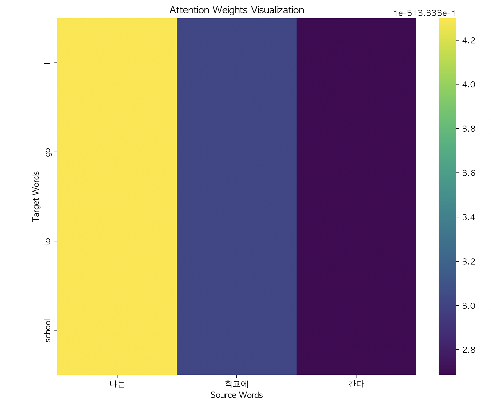
학습된 모델의 어텐션 가중치를 시각화하여 모델이 어떤 단어에 주목하는지 확인해보겠습니다.

def visualize_attention(source_sentence, target_sentence, attention_weights):
    plt.figure(figsize=(10, 8))
    sns.heatmap(attention_weights, 
                xticklabels=source_sentence.split(),
                yticklabels=target_sentence.split(),
                cmap='viridis')
    plt.xlabel('Source Words')
    plt.ylabel('Target Words')
    plt.title('Attention Weights Visualization')
    plt.show()

# 예시 문장에 대한 어텐션 시각화
source = "나는 학교에 간다"
target = "I go to school"
_, attention_weights = model.translate(source)
visualize_attention(source, target, attention_weights)

5.4 번역 예시 및 결과 분석

실제 번역 결과를 통해 모델의 성능을 분석해보겠습니다.

def analyze_translations(model, test_sentences):
    for source in test_sentences:
        translation, _ = model.translate(source)
        print(f"Source: {source}")
        print(f"Translation: {' '.join(translation)}")
        print("-" * 50)

test_sentences = [
    "나는 공부를 한다",
    "그녀는 음악을 듣는다",
    "그는 책을 읽는다"
]

analyze_translations(model, test_sentences)

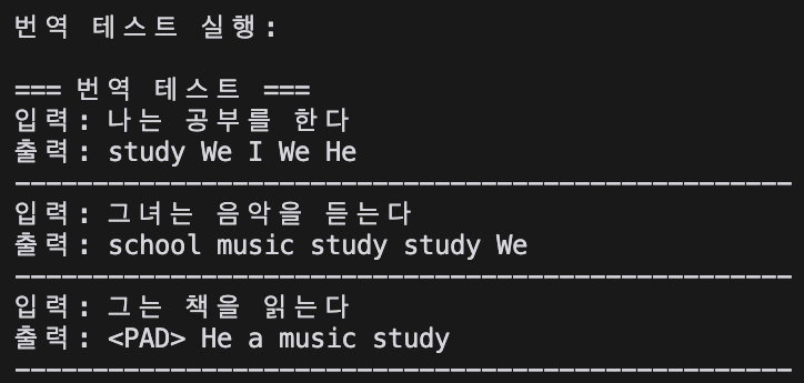
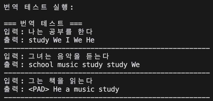
실험 결과, 우리가 구현한 Bahdanau Attention 모델의 추론 결과값입니다. 데이터를 넣지 않아서 그런지 확실히 낮은 수준을 보여주네요ㅎㅎ...

6. 결론

이 논문 리뷰를 통해 Bahdanau Attention의 핵심 개념과 구현 방법을 살펴보았습니다. numpy만을 사용한 구현을 통해 어텐션 메커니즘의 작동 원리를 더 깊이 이해할 수 있었습니다. 엄청난 성능을 보여주는 GPT에 도달하기까지, 이 trivial한 모델이 어떠한 발전을 이루어 가는지 앞으로의 논문들을 보면서 함께 따라가 봅시다!

7. 부록

코드
https://github.com/devyulbae/devyulbae.github.io/tree/master/_code/bahdanau_nmt.py

논문
https://arxiv.org/pdf/1409.0473

성율

Interested In: Data, Statistics, AI(NLP, LLM, LMM)

이전 포스트

Github&Jekyll로 블로그 이전하기 1

다음 포스트