92일차 시작.... (LogisticRegression)
1. 혼동 행렬 추출 방법2-1. [방법1] 기본 성능 지표 구하기2-2. [방법2] 기본 성능 지표 구하기3. FPR, TPR 구하기4. ROC 곡선 그래프 그리기5. AUC - ROC 곡선 면적값 구하기LogisticRegression 학습 전개classification_report 메소드 사용sklearn 다중 분류 전개sklearn의 LogisticRegression다중 분류 모델 - sklearn분류 정확도 성능 지표
[교육] Python ML
목록 보기
7/17

📊 sklearn의 LogisticRegression
📌 LogisticRegression 학습 전개
- 1. 라이브러리 Import
import pandas as pd
import numpy as np
import matplotlib.pyplot as plt
import seaborn as sns
from sklearn.preprocessing import MinMaxScaler
from sklearn.model_selection import train_test_split
from sklearn.linear_model import LogisticRegression
from sklearn.metrics import accuracy_score
- 2. 데이터 준비
data = pd.read_csv('../testdata/pima-indians-diabetes.data.csv', header=None)
data.columns = ['Pregnancies','Glucose','BloodPressure','SkinThickness','Insulin','BMI', 'DiabetesPedigreeFunction', 'Age','Outcome']
print(data.head(3))
#    Pregnancies  Glucose  BloodPressure  ...  DiabetesPedigreeFunction  Age  Outcome
# 0            6      148             72  ...                     0.627   50        1
# 1            1       85             66  ...                     0.351   31        0
# 2            8      183             64  ...                     0.672   32        1
- 3. 학습, 테스트 데이터 분리
train, test = train_test_split(data, test_size=0.3, random_state=1)
x_train = train.iloc[:, :-1]
y_train = train.iloc[:, -1]
x_test = test.iloc[:, :-1]
y_test = test.iloc[:, -1]
print(len(x_train), len(x_test))
# 537 231
# -> 7:3 비율로 분리
- 4. sklearn 모델에 사용하기 위해 배열 형태로 feature, label 분리
x = np.array(x_train)
y = np.array(y_train)
print(x.shape, y.shape)
# (537, 8) (537,)
# x : 537행 8열    - 2차원 Matrix
# y : 537개        - 1차원 Vector
- 5. sklearn 로지스틱회귀 모델 학습
model = LogisticRegression()
model.fit(x, y)
- 6. 예측값, 실제값 비교
x_test = np.array(x_test)
y_test = np.array(y_test)
y_pred = model.predict(x_test)
print('실제값 : ', y_test[:3])
print('예측값 : ', y_pred[:3])
# 실제값 :  [0 0 0]
# 예측값 :  [0 0 0]
- 7. 모델 성능 평가
print('학습세트 정확도 : ', accuracy_score(y, model.predict(x)))
print('테스트세트 정확도 : ', accuracy_score(y_test, y_pred))
# 학습세트 정확도 :  0.7728119180633147
# 테스트세트 정확도 :  0.7835497835497836
- 8. 모델 성능 평가 결과분석
[ 학습, 테스트 정확도 간의 차이가 많이 나면 학습데이터에 대해 과적합된 것을 의미함 ]
→ 과적합 되지 않음
→ 78.3% 정도의 성능 추출
📊 다중 분류 모델
📌 다중 분류 모델 - sklearn
- sklearn 로지스틱회귀 모델 특징
- 이진분류, 다중분류 기능을 제공하기 위해 일반화되어 있다.
📌 sklearn 다중 분류 전개
- 1. 라이브러리 Import
- MinMaxScaler : feature 정규화
- StandardScaler : feature 표준화
- LabelEncoder : label 인코딩(범주형 -> 숫자형)import pandas as pd import numpy as np import matplotlib.pyplot as plt import seaborn as sns from sklearn.preprocessing import MinMaxScaler, StandardScaler, LabelEncoder from sklearn.model_selection import train_test_split from sklearn.linear_model import LogisticRegression from sklearn.metrics import accuracy_score
- 2. 데이터 준비
data = pd.read_csv('../testdata/iris.csv')
print(data.head(3))
#    Sepal.Length  Sepal.Width  Petal.Length  Petal.Width Species
# 0           5.1          3.5           1.4          0.2  setosa
# 1           4.9          3.0           1.4          0.2  setosa
# 2           4.7          3.2           1.3          0.2  setosa
- 3. 상관관계 분석
print(data.corr())
#               Sepal.Length  Sepal.Width  Petal.Length  Petal.Width
# Sepal.Length      1.000000    -0.117570      0.871754     0.817941
# Sepal.Width      -0.117570     1.000000     -0.428440    -0.366126
# Petal.Length      0.871754    -0.428440      1.000000     0.962865
# Petal.Width       0.817941    -0.366126      0.962865     1.000000
[ 상관관계 분석 결과 ]
Petal.Length - Petal.Width : 0.962865
Sepal.Length - Petal.Length : 0.871754
Sepal.Length - Petal.Width : 0.817941
→ 상관계수가 가장 강한 Petal.Length, Petal.Width 선택
- 4. 사용 칼럼 추출
data = data.loc[:, ['Petal.Length', 'Petal.Width', 'Species']]
print(data.head(3))
#    Petal.Length  Petal.Width Species
# 0           1.4          0.2  setosa
# 1           1.4          0.2  setosa
# 2           1.3          0.2  setosa
- 5. label Encoding - 범주형 label에서 숫자형 label로 인코딩
x = np.array(data.iloc[:, :-1])
y = np.array(data.iloc[:, -1])
encoder = LabelEncoder()
y = encoder.fit_transform(y)
print(y[:3])
# [0 0 0]
- 6. 학습, 테스트 데이터 분리
x_train, x_test, y_train, y_test = train_test_split(x, y, test_size=0.3, random_state=1)
print(x_train.shape, x_test.shape)
# (105, 2) (45, 2)
- 7. 다중 분류 모델(로지스틱회귀)
model = LogisticRegression(C=1.0, random_state=0)   # C 속성 : 모델에 정규화(L2) 규제를 적용 -> 학습 과소, 과대적합을 해소하기 위한 장치
model.fit(x_train, y_train)
- 8. 모델 예측값, 실제값 비교
y_pred = model.predict(x_test)
print('실제값 : ', y_test[:3])
print('예측값 : ', y_pred[:3])
# 실제값 :  [0 1 1]
# 예측값 :  [0 1 1]
- 9. 모델 성능 평가
print('학습데이터 분류 정확도 : ', accuracy_score(y_train, model.predict(x_train)))
print('검정데이터 분류 정확도 : ', accuracy_score(y_test, y_pred))
# 학습데이터 분류 정확도 :  0.9714285714285714
# 검정데이터 분류 정확도 :  0.9777777777777777
# -> 과적합 없음
# -> 97%의 분류 정확도
📊 분류 모델 정확도 성능 지표 전개
📌 분류 정확도 성능 지표
- 혼동 행렬
- 기본 성능 지표
1) 정확도(accuracy) = (TP + TN) / 전체개수
2) 재현도(recall) = TP / (TP + FN)
3) 정밀도(presision) = TP / (TP + FP)
- FPR(False Positive Rate), TPR(True Positive Rate)
4) FPR : 거짓 양성 비율 = FP / (FP + TN)
5) TPR : 참 양성 비율 = TP / (TP + FN)
- 6) ROC 곡선 - 그래프 사용
- x축 : FPR
- y축 : TPR
- 7) AUC 지표
- ROC 면적을 통해 구하기
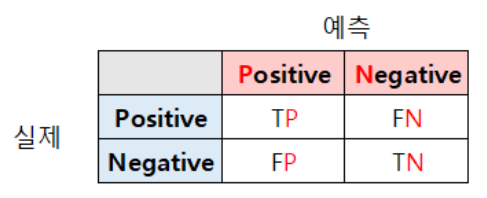
📌 1. 혼동 행렬 추출 방법
- 0. 필요 인자값
실제값과 예측값을 이용해서 추출 가능
- 1. 필요 라이브러리
- sklearn.metrics에서 제공하는 confusion_matrix 메소드를 사용한다.from sklearn.metrics import confusion_matrix
- 2. 혼동 행렬 추출
- confusion_matrix(실제값, 예측값)
→ crosstab으로 만들 수 있지만 sklearn에서 제공하는 메소드 사용이 편리함conf = confusion_matrix(y_test, y_pred) print(conf) # [[153 4] # [ 9 131]] TP = 153 FN = 4 FP = 9 TN = 131
- 3. 혼동 행렬 분석
- TP = 153 -> conf[0][0]
- FN = 4 -> conf[0][1]
- FP = 9 -> conf[1][0]
- TN = 131 -> conf[1][1]
📌 2-1. [방법1] 기본 성능 지표 구하기
[ 수기로 구하기 ]
- 1. 혼동행렬을 이용한 정확도 구하기
accuracy = (TP + TN) / len(y_test)
print('acc : ', accuracy)
# 정확도 :  0.9562289562289562
- 2. 혼동행렬을 이용한 재현도 구하기
recall = TP / (TP + FN)
print('재현도 : ', recall)
# 재현도 :  0.9745222929936306
- 3. 혼동행렬을 이용한 정밀도 구하기
presision = TP / (TP + FP)
print('정밀도 : ', presision)
# 정밀도 :  0.9444444444444444
📌 2-2. [방법2] 기본 성능 지표 구하기
[ classification_report 메소드 사용 ]
- 1. 필요 라이브러리
from sklearn.metrics import classification_report
- 2. 분류 종합 성능 자료 출력
report = classification_report(y_test, y_pred)
print(report)
#               precision    recall  f1-score   support
#
#            0       0.94      0.97      0.96       157
#            1       0.97      0.94      0.95       140
#
#     accuracy                           0.96       297
#    macro avg       0.96      0.96      0.96       297
# weighted avg       0.96      0.96      0.96       297
# -> 정확도 : 0.96
# -> 정밀도 : 0.94
# -> 재현도 : 0.97
📌 3. FPR, TPR 구하기
- 1. 필요 라이브러리
from sklearn.metrics import roc_curve
- 2. FPR, TPR 구하기
FPR, TPR, _ = roc_curve(y_test, y_pred)
print('거짓 양성 비율 : ', FPR)
print('진 양성 비율 : ', TPR)
# 거짓 양성 비율 :  [0.         0.02547771 1.        ]
# 진 양성 비율 :  [0.         0.93571429 1.        ]
📌 4. ROC 곡선 그래프 그리기
- 1. ROC curve 그래프 전개
plt.plot(FPR, TPR, label='Logistic Regression')
plt.plot([0, 1], [0, 1], '--', label='ROC curve - AUC(0.5) area')
plt.xlabel('False Positive Rate')
plt.ylabel('True Positive Rate')
plt.title('ROC curve')
plt.show()
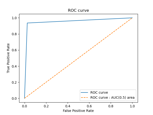
📌 5. AUC - ROC 곡선 면적값 구하기
- 1. 필요 라이브러리
from sklearn.metrics import auc
- 2. AUC 면적값 구하기
auc_value = auc(FPR, TPR)
print('AUC : ', auc_value)
# AUC 면적 :  0.9551182893539581
# -> 매우 높은 AUC 비율을 보인다.
# -> 모델 성능이 매우 높음

데이터 사이언티스트를 목표로 하는 개발자