[논문 준비] - 불균형 데이터 처리

불균형 데이터(Imbalanced data)

• 클래스 간의 데이터 수가 균일하게 분포되어 있지 않은 경우를 말한다.
  • 의료데이터의 경우 데이터셋 내에서 발병율에 따라 클래스 불균형이 필연적으로 발생
  • 신용카드 사용자의 사기탐지 경우, 정상 거래가 비정상 거래보다 훨씬 많다.

📌 문제점

• 소수 클래스에 속한 데이터들은 다수 클래스에 속한 데이터보다 오분류될 가능성이 높다
• 정확도가 높더라도 재현율 또는 민감도가 낮아질 수 있다.

불균형 데이터를 해결하기 위한 방법

• 두 클래스중 어느 클래스의 데이터 수를 조절하느냐에 따라 언더샘플링 기법과 오버샘플링 기법으로 분류할 수 있다.

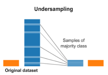
1. 언더샘플링(Under sampling)

• 언더샘플링은 소수 클래스의 데이터 수에 맞도록 다수 클래스의 데이터를 제거하는 방식

• 언더샘플링 기법들은 데이터를 제거함으로 정보가 손실되는 문제점이 있다.

• 랜덤 언더샘플링(Random Under-sampling), Tomek-links, EasyEnsemble 등의 기법이 존재

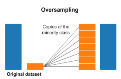
2. 오버 샘플링(Over sampling)

• 다수 클래스 데이터 수에 맞춰 소수 클래스의 데이터를 생성하는 방식

• 정보 손실을 해결할 수 있지만, 데이터의 증가로 인한 계산 시간 증가, 과적합 등의 문제가 발생할 수 있다.

• 랜덤 오버샘플링, SMOTE, ADASYN (He, H. 등, 2008), Borderline-SMOTE 등의 다양한 기법이 존재

2-1. 오버샘플링 기법

1) 랜덤 오버샘플링

• 다수 클래스의 표본 크기와 같아질 때까지 소수 클래스의 표본을 무작위로 반복 복원 추출시키는 방법
• 소수 클래스의 표본 수는 증가하지만, 단순히 소수 클래스의 표본을 복제하는 것이기 때문에 표본이 중복된다.

2) SMOTE (Synthetic Minority Oversampling Technique)

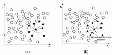
• k-NN 알고리즘을 활용하여 소수 클래스 임의의 표본을 중심으로 k개의 최근접 이웃을 합성하여 선형 연결 구조 사이에 합성 표본을 생성
• ROS의 같은 표본의 중복으로 인한 과적합 문제를 보완한다.

3) Borderline-SMOTE

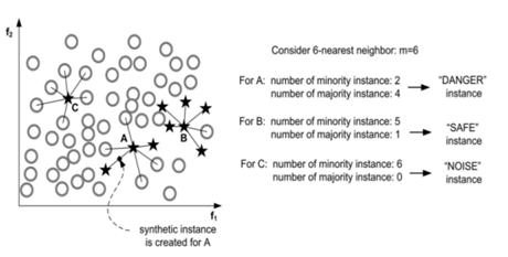
• SMOTE를 확장한 방법으로, 두 클래스의 경계에 있는 값만을 이용하여 오버샘플링 한다.
• 다수 클래스의 표본 개수를 $N$이라고 할 때, 아래와 같은 집단으로 구분하여 "Danger" 집단에 속하는 소수 클래스의 표본에 대해서만 새로운 표본을 생성한다.

$Safe : 0 \le\ N\ < k/2$
$Danger : k/2 \le\ N\ < k$
$Noise : N=k$

4) ADASYN (Adaptive Synthetic Sampling)

• 소수 클래스의 표본마다 밀도 분포를 계산하고 이에 맞춰 생성할 표본의 개수를 결정하여 생성하는 방법
• 각 관측치마다 생성하는 샘플의 수가 다르다는 점이 특징

오버샘플링 실습

• 자료 : Breast Cancer Wisconsin (Diagnostic) Data Set (.csv)
• target 변수 : diagnosis (M = malignant, B = benign)
• dataset을 임의로 불균형하게 조절하였다.

Library Import

import numpy as np 
import pandas as pd # data processing, CSV file I/O (e.g. pd.read_csv)
import matplotlib.pyplot as plt
import seaborn as sns
from collections import Counter

Load data

data = pd.read_csv('wisconsin dataset.csv')
data['diagnosis'] = data['diagnosis'].replace({'M' : 1 , 'B' : 0}) # M을 1로, B를 0으로 바꿔줌
data.head()

X = data.drop(columns={'diagnosis'})
y = data['diagnosis']

y_count = data['diagnosis'].value_counts()
print(y_count)

0    357
1     38
Name: diagnosis, dtype: int64

IR이 약 9.4 (IR=357/38=9.3947)로 심한 불균형을 보인다.

fig = sns.countplot(data['diagnosis'])
fig.set_xticklabels(['Benign(0)', 'Malignant(1)'])
plt.show()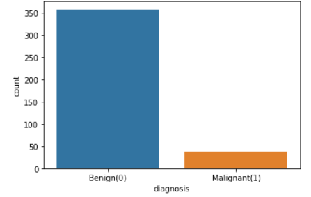

oversampling method

1. Random oversampling

from imblearn.over_sampling import RandomOverSampler
counter = Counter(y)
print('Before',counter)
ros = RandomOverSampler(random_state=0)
x_ros, y_ros = ros.fit_resample(X, y)
counter = Counter(y_ros)
print('After',counter)

# 결과
Before Counter({0: 357, 1: 38})
After Counter({1: 357, 0: 357})

# df_ros로 만들어줌
df_ros = x_ros.copy()
df_ros['y'] = y_ros

2. SMOTE

from imblearn.over_sampling import SMOTE
counter = Counter(y)
print('Before',counter)
smote = SMOTE(random_state=0)
x_smote, y_smote = smote.fit_resample(X,y)
counter = Counter(y_smote)
print('After',counter)

# 결과
Before Counter({0: 357, 1: 38})
After Counter({1: 357, 0: 357})

# df_smote로 만들어줌
df_smote = x_smote.copy()
df_smote['y'] = y_smote

3. BorderlineSMOTE

from imblearn.over_sampling import BorderlineSMOTE
counter = Counter(y)
print('Before',counter)
B_SMOTE = BorderlineSMOTE(random_state=0)
x_b_smote, y_b_smote = B_SMOTE.fit_resample(X, y)
counter = Counter(y_b_smote)
print('After',counter)

# 결과
Before Counter({0: 357, 1: 38})
After Counter({1: 357, 0: 357})

# df_b_smote로 만들어줌
df_b_smote = x_b_smote.copy()
df_b_smote['y'] = y_b_smote

4. ADASYN

from imblearn.over_sampling import ADASYN
counter = Counter(y)
print('Before',counter)
adasyn = ADASYN(random_state=0)
x_adasyn, y_adasyn = adasyn.fit_resample(X, y)
counter = Counter(y_adasyn)
print('After',counter)

# 결과
Before Counter({0: 357, 1: 38})
After Counter({0: 357, 1: 353})

# df_adasyn로 만들어줌
df_adasyn = x_adasyn.copy()
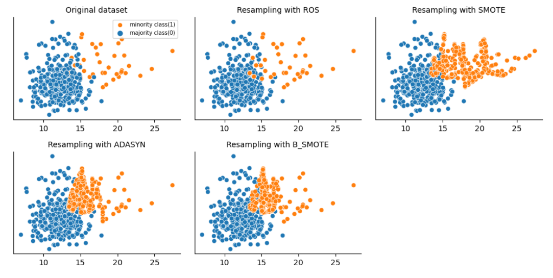
df_adasyn['y'] = y_adasyn

Data visualization

f, axes = plt.subplots(2,3,figsize=(10, 5), dpi=100)
sns.despine()
sns.scatterplot(x='radius_mean', y='texture_mean', hue = y, data=data, ax=axes[0,0])
axes[0,0].set_title('Original dataset', fontsize=10)
axes[0,0].legend(['minority class(1)', 'majority class(0)'], fontsize=7)
axes[0,0].set_xlabel(None)
axes[0,0].set_ylabel(None)
sns.scatterplot(x='radius_mean', y='texture_mean', hue = 'y', data=df_ros, ax=axes[0,1], legend=False)
axes[0,1].set_title('Resampling with ROS', fontsize=10)
axes[0,1].set_xlabel(None)
axes[0,1].set_ylabel(None)
sns.scatterplot(x='radius_mean', y='texture_mean', hue = 'y',data=df_smote, ax=axes[0,2], legend=False)
axes[0,2].set_title('Resampling with SMOTE', fontsize=10)
axes[0,2].set_xlabel(None)
axes[0,2].set_ylabel(None)
sns.scatterplot(x='radius_mean', y='texture_mean',hue = 'y', data=df_adasyn, ax=axes[1,0], legend=False)
axes[1,0].set_title('Resampling with ADASYN', fontsize=10)
axes[1,0].set_xlabel(None)
axes[1,0].set_ylabel(None)
sns.scatterplot(x='radius_mean', y='texture_mean', hue = 'y', data=df_b_smote, ax=axes[1,1], legend=False)
axes[1,1].set_title('Resampling with B_SMOTE', fontsize=10)
axes[1,1].set_xlabel(None)
axes[1,1].set_ylabel(None)
plt.setp(axes, yticks=[])
plt.tight_layout()
plt.show()