라이브러리 불러오기
import pandas as pd
import tensorflow as tf
import numpy as np
경사 설정, y = 2w^2+5
w = tf.Variable(2.)

def f(w):
    y = w**2
    z = 2*y + 5
    return z
with tf.GradientTape() as tape:
z = f(w)
gradient = tape.gradient(z, [w])
print(gradient)#w=4, b=1로 임의 설정
w = tf.Variable(4.0)
b = tf.Variable(1.0)선형회귀 식
def hypothesis(x):
    return w*x + b
# 테스트 식
x_test = [3.5, 5, 5.5, 6]
print(hypothesis(x_test).numpy())
[15. 21. 23. 25.]#손실함수 정의 MSE
def mse_loss(y_pred, y):
return tf.reduce_mean(tf.square(y_pred - y))# 학습 시간과 성적 데이터
x = [1, 2, 3, 4, 5, 6, 7, 8, 9]
y = [11, 22, 33, 44, 53, 66, 77, 87, 95]# 경사 학습률 0.01로
optimizer = tf.optimizers.SGD(0.01)#300번의 학습
for i in range(301):
with tf.GradientTape() as tape:
y_pred = hypothesis(x)
cost = mse_loss(y_pred, y)
gradients = tape.gradient(cost, [w, b])
optimizer.apply_gradients(zip(gradients, [w,b]))
if i % 10 ==0:
print("epoch : {:3} | w의 값 : {:5.4f} | b의 값 : {:5.4} | cost : {:5.6f}".format(i, w.numpy(), b.numpy(), cost))
Cost 줄어드는 모습 확인 가능
x_test = [3.5, 5, 5.5 ,6]
print(hypothesis(x_test).numpy())
[38.35479  54.295143 59.608593 64.92204 ]
케라스로
import numpy as np
import matplotlib.pyplot as plt
from tensorflow.keras.models import Sequential
from tensorflow.keras.layers import Dense
from tensorflow.keras import optimizers
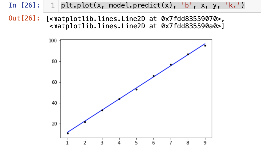
x = [1, 2, 3, 4, 5, 6, 7, 8, 9] # 공부하는 시간
y = [11, 22, 33, 44, 53, 66, 77, 87, 95] # 각 공부하는 시간에 맵핑되는 성적
model = Sequential()
model.add(Dense(1, input_dim = 1, activation = 'linear'))
sgd = optimizers.SGD(lr=0.01)
model.compile(optimizer=sgd, loss='mse', metrics=['mse'])
model.fit(x, y, epochs=300)
plt.plot(x, model.predict(x), 'b', x, y, 'k.')

데이터 사이언스를 공부하는 커피쟁이