Image ProcessingⅠ

Image Formation

Pinhole camera

• 카메라로 이미지를 얻는 과정은 복잡함
• pinhole camera model은 core concept in a simplified manner로 설명하는 것을 도와줌
  

Digital transformation

Sampling

이미지를 M x N grid of pixels로 만듦

Quantizing

픽셀의 값을 L(e.g. 256) discrete levels로 정함

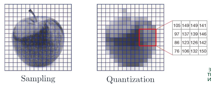
We can think of an image as a function
$f: R^2 → R$
$f(x,y)$ gives the intensity $\in [0, L - 1]$ at position (x,y)

color image는 three functions pasted together된 것임
$f(x,y)=\begin{bmatrix}r(x,y)\\g(x,y)\\b(x,y)\end{bmatrix}$

RGB color model

보통 각각 픽셀 값을 0~255의 값으로 표현함

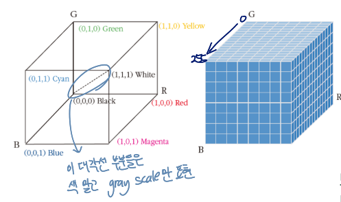
아는 내용이니까 이 정도만 짚고 넘어가도록 함

HSV color model

색의 타입, 밝기, 채도를 통해 색을 표현하는 방법

• H : Hue 색의 타입
• S : Saturation 채도
• V : brightness of light 밝기

More robust to changes in lighting compared to the RGB model

RGB vs. HSV

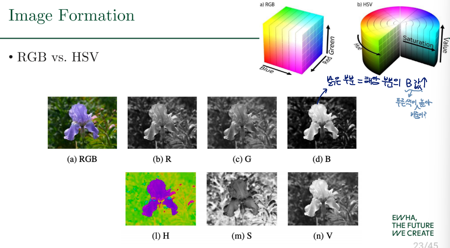
Image Processing

Existing image $f$로부터 새로운 이미지인 $g$를 만들고자 함

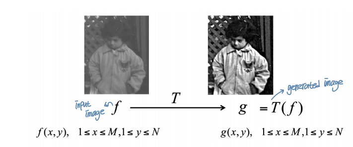
이런 것을 수행하기 위한 operation에는 어떤 것들이 있는지 알아볼 것임

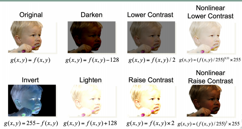
Point Operations

output pixel의 value는 오직 corresponding input pixel의 value에만 depends

위치를 나타내는 변수 $x=(i,j)$라고 한다면

$g(x) = T(f(x))\quad or\quad g(x) = T(f_0(x), f_1(x),...,f_n(x))$

뒤의 수식의 예 : RGB value인 경우 $g(x)=T(f_R(x), f_G(x), f_B(x))$

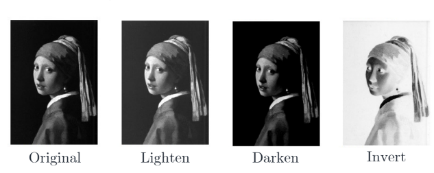
Linear operations

$g(j,i)=\begin{cases}min(f(j,i)+\alpha, L-1) &\text{Lighten}\\ max(f(j,i)-\alpha, 0) &\text{Darken}\\ (L-1)-f(j,i) &\text{Invert}\end{cases}$

이때, $\alpha$는 양수

Gamma correction

$g(j,i) = \begin{cases}(L-1) \times (\hat{f}(j,i))^\gamma &\text{where} \hat{f}(j,i) = \frac{f(j,i)}{(L-1)}\end{cases}$

• $\gamma = 1$ → identity function (=original image)
• $\gamma > 1→{\hat{f}(j,i)}^{\gamma} \leq 1$ → darken image
• $\gamma < 1→{\hat{f}(j,i)}^{\gamma} \geq 1$ → lighter image

$\gamma$를 역수 취하면 반대 결과를 얻게 됨

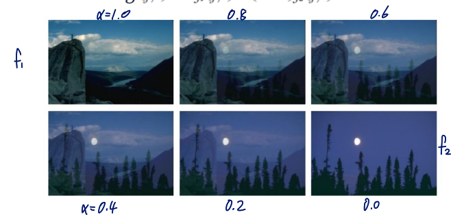
Scene dissolve

e.g. k=2
$g(j,i)=\alpha f_1(j,i) + (1-\alpha)f_2(j,i)$

Histogram

shows how often each (grayscale) value in the range [0, L-1] appears in the image

$h(l) = |\{(j,i)|f(j,i)=l\}|$ absolute count

$\hat{h}(l) = \frac{h(l)}{M \times N}$ normalized histogram

히스토그램을 통해 이미지의 특징을 파악할 수 있음
such as constrast, brightness, and intensity distribution

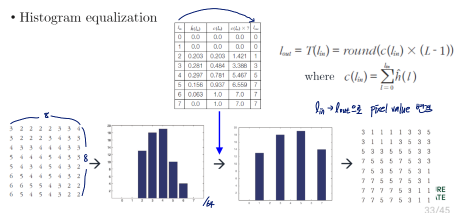
Histogram equalization

한국어로 평활화

• An operation that flattens the histogram
• Enhances image quality by expanding the dynamic range of intensities
• Uses the cumulative histogram, $c(\cdot)$, as the mapping function

$l_{out} = T(l_{in}) = round(c(l_{in}) \times (L-1))$
where $c(l_{in} = \sum_{l=0}^{l_{in}}\hat{h}(l))$

histogram equalization을 통해 이미지가 더 선명해짐

벌레가 더 잘 보이게 되었지만 texture가 별로임
→ histogram equalization을 사용하는 것이 언제나 좋은 것은 아님

Binarization (Thresholding)

$b(j,i) = \begin{cases} 1, & \text{f(j,i)} \geq T \\0, & \text{f(j,i)}) < T \end{cases}$

• Threshold를 어떻게 automatically 찾을 수 있을까?
  보통 valley 부분을 Threshold로 설정함
• What if there are more than one valley?
  Otsu's algorithm

Otsu's algorithm

• Based on the principle that binarization is better when both the black and white groups are as homogeneous as possible
  black과 white pixel의 비율이 비슷해야 한다는 뜻인듯?
• Homogeneity is measured by variance: lower variance within each group indicates higher homogeneity
  variance를 통해 homogeneity가 측정되는데, 각각 그룹의 variance가 낮을수록 homogeneity는 높음

$T= \underset{t\in \{0,1,...,L-1\}}{\mathrm{argmin}} v_{within}(t)$

$v_{within}(t) = w_0(t)v_0(t)+w_1(t)v_1(t)$

$w_0(t) = \underset{i=0}{\overset{t}{\sum}}\hat{h}(i)$          $w_1(t) = \underset{i=t+1}{\overset{L-1}{\sum}}\hat{h}(i)$

$\mu_0(t) = \frac{1}{w_0(t)}\underset{i=0} {\overset{t}{\sum}}i\hat{h}(i)$         $\mu_1(t) = \frac{1}{w_1(t)}\underset{i=t+1} {\overset{L-1}{\sum}}i\hat{h}(i)$

$v_0(t) = \frac{1}{w_0(t)}\underset{i=0} {\overset{t}{\sum}}\hat{h}(i)(i-\mu_0(t))^2$   $v_1(t) = \frac{1}{w_1(t)}\underset{i=t+1} {\overset{L-1}{\sum}}\hat{h}(i)(i-\mu_1(t))^2$

그러나 시간복잡도가 $O(L^2)$으로 매우 느리다는 단점을 갖고 있음
argmin을 구하는 횟수 L번, 각 $v_{within}(t)$를 구할 때 계산량 $O(L)$ → $O(L^2)$

efficient veresion
$v = \underset{i=0}{\overset{L-1}{\sum}}(i-\mu)^2\hat{h}(i) = v_{within} + v_{between}$

$where$  $v_{within}(t) = w_0(t)v_0(t) + w_1(t)v_1(t)$
     $v_{between}(t) = w_0(t)(1-w_0(t))(\mu_0(t)-\mu(t))^2$
                    각 그룹 평균의 차로 define

$\therefore \quad T= \underset{t \in \{0,1,...,L-1\}}{\mathrm{argmin}}v_{within}(t) \quad \leftrightarrow\quad$ $T= \underset{t \in \{0,1,...,L-1\}}{\mathrm{argmax}}v_{between}(t)$

$w_0(t) = w_0(t-1)+\hat{h}(t)$
$\mu_0(t) = \frac{w_0(t-1)\mu_0(t-1+t\hat{h}(t))}{w_0(t)}$
$\mu_1(t) = \frac{\mu - w_0(t)\mu_0(t)}{1-w_0(t)}$
→ 이전에 구해놓은 값들을 사용하면 바로 구할 수 있음
→ recycle previous value를 통해 일일이 계산 안해도 되게 됨!

여러 point operations 결과