Lecture 9 : Sort

Sorting

lists a set of data in ascending or descending order

Sorting is essential whe searching data
Ex) What if words in the English dictionary are not sorted alphabetically?

Target of Sorting

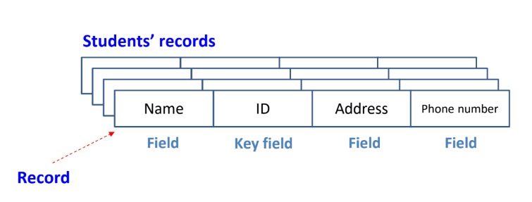
Record

1. Data to be sorted
2. Consists of multiple fields
3. Key field is used to identify records
   

Sorting Algorithm

No golden solution that workds for all cases perfectly

Sorting algorithm must be chosen by considering the following cases

• the number of records(data)
• record size
• key characteristics(letter, integer, floating number)
• internal / external memory sorting
  trade off : memory↑, speed↓ / memory↓, speed↑

Evaluation criteria of sorting algorithm

1. the number of comparisons
2. the number of moves of data

Summary of Sorting Algorithms

	Best	Average	Worst	Stability
Insert sort	O(n)	O(n²)	O(n²)	Yes
Selection sort	O(n²)	O(n²)	O(n²)	No
Bubble sort	O(n²)	O(n²)	O(n²)	Yes
Shell sort	O(n)	O(n^1.5)	O(n^1.5)	No
Quick sort	O(nlog₂n)	O(nlog₂n)	O(n²)	No
Heap sort	O(nlog₂n)	O(nlog₂n)	O(nlog₂n)	No
Merge sort	O(nlog₂n)	O(nlog₂n)	O(nlog₂n)	Yes
Count sort	O(n)	O(n)	O(n)	Yes
Radix sort	O(dn)	O(dn)	O(dn)	Yes

Insert sort ~ Bubble sort : not using devide and conquer (=간단한 sorting 방법)
Quick sort ~ Merge sort : devide and conquer
Count sort, Radix sort : integer sorting

Simple but inefficient algorithms

insert sort, selection sort, bubble sort

Complex but efficient algorithms

quick sort, heap sort, merge sort, radix sort

Internal sort

Sort a set of data that is stored in main memory

External sort

Sort a set of data, when most of the data is stored in the external storage device and only a part of the data is stored in the main memory

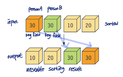
Stability of sorting algorithm

The relative position of records with the same key value does not change after sorting

Example of unstable sort

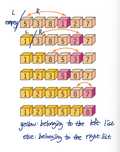
Selection Sort

An input array : left and right lists

• left list : sorted data
• right list : unordered data
• initially, the left list is empty, and all the numbers to sort are in the right list

Procedure

1. Select the minimum value in the right list and exchange it with the first number of right list
2. Increase the left list size
3. Decrease the right list size

Iterate 1-3 until the right list is empty

Pseudo code

selection_sort(A, n)

for i←0 to n-2 do
	least ← an index of the smallest value among A[i], A[i+1],...,A[n-1];
    Swap A[i] and A[least];
    i++;

C code

#define SWAP(x, y, t) ( (t)=(x), (x)=(y), (y)=(t) )

void selection_sort(int list[], int n){
	int i, j, least, temp;
    for(i=0; i<n-1; i++){
    	least = i;
        for(j=i+1; j<n; j++){
        	if(list[j]<list[least]) 
            	least = j;
        }
        SWAP(list[i], list[least], temp);
    }
}

• # of comparisons : (n-1)+(n-2)+...+1 = n(n-1)/2 = O(n²)
• # of moves : 3(n-1)
• Time complexity : O(n²)
• The selection sort is not stable
  

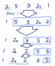
Insertion Sort

Iteratively insert a new record in the right place the sorted part

Pseudo code

insertion_sort(A, n)

1. for i←1 to n-1 do
2.		key ← A[i];
3. 		j ← i-1;
4. 		while j>=0 and A[j]>key do
5.			A[j+1]←A[j];
6.			j←j-1;
7. 		A[j+1] ← key

Procedure

1. Starting from i=1
2. Copy the i-th integer, which is the current number to insert, into the key variable
3. Start at (i-1)-th position, since the currently sorted array is up to i-1
4. If the value in the sorted array is greater than the key value,
5. Move the j-th data to the (j+1)-th data
6. Decrease j
7. Because the j-th integer is less than key, copy the key into the (j+1) position

C code

void insertion_sort(int list[], int n){
	int i, j, key;
    for(i=1; i<n; i++){
    	key = list[i];
        for(j=i-1; j>=0 && list[j]>key; j--)
        	list[j+1] = list[j];
        list[j+1] = key;
    }
}

Time Complexity of Insert Sort

Best case : when the data is already sorted

• # of comparisons: n-1
• # of moves : 0

Wort case : when sorted in reverse order

• # of comparisons : ∑(i=1~n-1) i = n(n-1)/2 = O(n²)
• # of moves : n(n-1)/2 + 2(n-1) = O(n²)

Property

• when the data size is large, the time complexity increases significantly
• Stable sort
• It is very efficient when the data is mostly sorted

Bubble Sort

Procedure

1. Swap two adjacent data, when they are not in order
2. This comparison-exchange process is repeated from the left to the right

Pseudo code

BubbleSort(A, n)

for i←n-1 to 1 do
	for j←0 to i-1 do
    	Swap if when j and j+1 elements are not in order
        j++;
        
    i--;

C code

#define SWAP(x,y,t) ((t)=(x), (x)=(y), (y)=(t))
void bubble_sort(int list[], int n){
	int i, j, temp;
    for(i=n-1; i>0; i--){
    	for(j=0; j<i; j++)
        	if(list[j]>list[j+1])
            	SWAP(list[j], list[j+1], temp);
    }
}

Time Complexity of Bubble Sort

Best case : when the data is already sorted

• # of comparisons: ∑(i=1~n-1) i = n(n-1)/2
• # of moves : 0
  near implement에서 중요해서 고려해야 함 ((t=x; x=y; y=t)하는 과정에 energy consumsion 발생)

Worst case : when sorted in reverse order

• # of comparisons: ∑(i=1~n-1) i = n(n-1)/2
• # of moves : 3*comparison count = 3∑(i=1~n-1) i = 3n(n-1)/2

It is stable sort

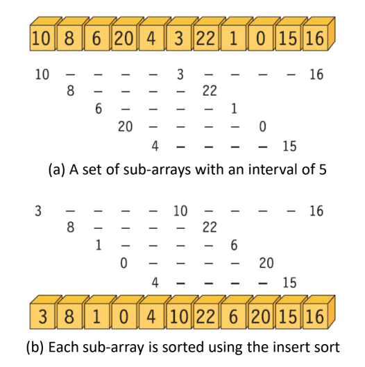
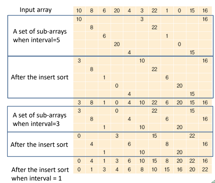
Shell Sort

Motivation

• Insert sort is very efficient when the data is mostly sorted
• the insertion sort moves elements only to neighboring positions
• by allowing elements to move to a remote location, they can be sorted with a smaller amount of moves

Procedure

1. Divide the array into a set of sub-arrays with an interval
2. Apply the insert sort to each sub-array
3. Decrease the interval

Iterate 1-3 until the interval becomes 1

C code

// Insert and sort elements apart by interval
//the range of sort is first to last
inc_insertion_sort(int list[], int first, int last, int gap){
	int i, j, key;
    for(i=first+gap; i<=last; i+=gap){
    	key = list[i];
        for(j=i-gap; j>=first && key<list[j]; j-=gap){
        	list[j+gap] = list[j];
        }
        list[j+gap] = key;
    }
}

//n= size
void sehll_sort(int list[], int n) {
	int i, gap;
    for(gap = n/2; gap>0; gap/=2){
    	if((gap%2)==0) gap++;
        for(i=0; i<gap; i++){
        	inc_insertion_sort(list, i, n-1, gap);
        }
    }
}

Advantages of shell sort

• Increases the likelihood of completing the sort with less amount of moves by moving remote data in a sub-array
• Since the sub-arrays become progressively sorted, the insertion sort becomes faster when the interval decreases

Time complexity

• Worst case : O(n²)
• Average case : O(n^1.5)

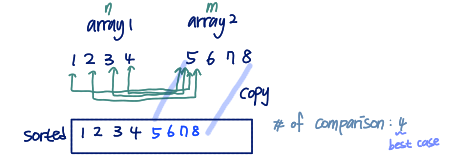
Merge Sort

Using the divide and conquer method

1. Divide the array into two equal sized and sort the split arrays
2. Sort the entire array by summing the two sorted arrays

Example
Input: (27 10 12 20 25 13 15 22)
1. Divide: divide it into (27 10 12 20) and (25 13 15 22)
2. Conquer: Sort the sub-arrays - (10 12 20 27) and (13 15 22 25)
3. Combine: Merge the sorted sub-arrays: (10 12 13 15 20 22 25 27)

Pseudo code

merge_sort(list, left, right)
1. 	if left<righta
2.		mid = (left+right)/2;
3.		merge_sort(list, left, mid);
4.		merge_sort(list, mid+1, right);
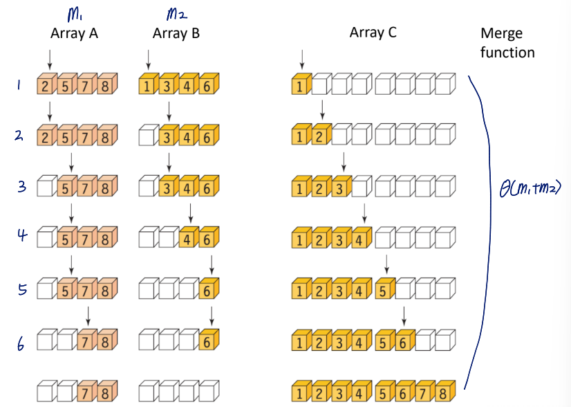
5.		merge(list, left, mid, right);

Procedure

1. If the size of the segment is greater than 1
2. Calculate intermediate position
3. Sort the left-side array(recursive call)
4. Sort the right sub-array(recursive call)
5. Merge the two sorted subarrays

Pseudo code

merge(list, left, mid, right)

i←left;
j←mid+1;
k←left;
while(i<=mid && j<=right) do
	if(list[i] <= list[j])
    	sorted[k]←list[i];
        k++;
        i++;
    else
    	sorted[k] ← list[j]
        k++;
        j++;

copies the remaining elements to 'sorted';
copy 'sorted' to list;

C code

int sorted[MAX_SIZE]

void merge(int list[], int left, int mid, int right){
	int i, j, k, l;
    i = left; j = mid+1; k = left;
    
    //merge split-sorted arrays
    while(i<=mid && j<=right){
    	if(list[i] <= list[j]){
        	sorted[k++] = list[i++];
        }
        else sorted[k++] = list[j++];
    }
    
    //right part에 복사 못한 데이터가 남아있는 경우
    if(i>mid){
    	for(l=i; l<=right; l++){
        	sorted[k++] = list[l];
        }
    }
    else{	//left part에 복사 못한 데이터 남아있는 경우
    	for(l=i; l<=mid; l++){
         	sorted[k++] = list[l];
        }
    }
    
    // sorted를 list에 복사
    for(l=left; l<=right; l++){
    	list[l] = sorted[l];
    }
}

void merge_sort(int list[], int left, int right){
	int mid;
    if(left<right){
    	mid = (left+right)/2;
        merge_sort(list, left, mid);
        merge_sort(list, mid+1, right);
        merge(list, left, mid, right);
    }
}

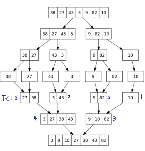
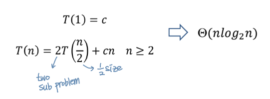
Time Complexity of Merge Sort

Totally, log₂n recursion

• For each recursion,
  • # of comparisons = n
  • # of moves = 2n

→ best and worst case : O(nlog₂n) and Ω(nlog₂n) => θ(nlog₂n)

Note

1. if the input is implemented using the linked list, the move becomes a simple address updae
2. it is a stable sort and is less influenced by the initial order of data

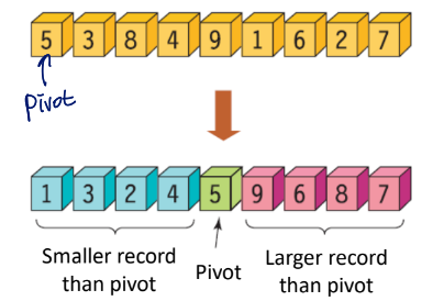
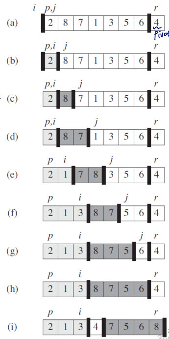
Quick Sort

Property

1. In average, the fastest sorting algorithm
2. Divide-and-conquer method
3. Unstable sort

Method

1. divide the array into two sizes using pivot
2. call the quick sort recursively
   

C code

void quick_sort(int list[], int left, int right){
	if(left<right){
    	int q=partition(list, left, right);
        quick_sort(list, left, q-1);
        quick_sort(list, q+1, right);
    }
}

1. if the size of the segment is greater than 1
2. partition into two lists based on pivot.
   the 'partiton' function returns the position of the pivot
3. recursive call from left to right before the pivot (except pivot)
4. recursive call from left next the pivot to right (except pivot)

partition function (less efficient one)

int partition(int list[], int left, int right){
	int pivot, temp;
    int low, high;
    
    low = left+1;
    high = right;
    pivot = list[left];
    while(low<high){
    	while(low<right && list[low]<pivot){
        	low++;
        }
        while(high>left && list[high]>pivot){
        	high--;
        }
        if(low<high) SWAP(list[low], list[high], temp);
    }
    
    SWAP(list[left], list[high], temp);
    return high;
}

partition function (more efficient one)

int partition(int list[], int left, int right){
	int temp;
	int x = A[right];	//pivot
    int i = left-1;
    
    for(int j=left; j<right; j++){
    	if(A[j]<=x){
        	i++;
            SWAP(A[i], A[j], temp);
        }
    }
    SWAP(A[i+1], A[right], temp);
    return i+1;
}

time complexity of this function: θ(n)

Time Complexity of Quick Sort

Best case

• when the array is partitioned almost equally
  pivot이 잘 선택된 경우
• # of recursions: _log₂_n
• # of comparisons for each recursion: n

=> θ(nlog₂n)

Worst case

• when the array is partitioned unequally
  empty left
• # of recursions: n
• # of comparisons for each recursion: n

=> θ(n²)
pivot을 랜덤하게 고르거나 중간값을 고르는 것이 솔루션이 될 수 있음!
.
.
.
+
pivot을 잘 고르면 merge보다 성능이 좋아서 더 많이 사용됨!

Sorting So Far

Comparison based sorting

• selection sort, insert sort, bubble sort, shell sort
• heap sort, merge sort, quick sort
• time complexity: n² or n_log₂_n

Non-comparison sorting is also possible

• counting sort, radix sort
• time complexity: n

Counting Sort

제한조건: 원소 type=integer, 원소 범위 알고 있어야 함
cumulated histogram(=cumulated destiny function=CDF) 사용

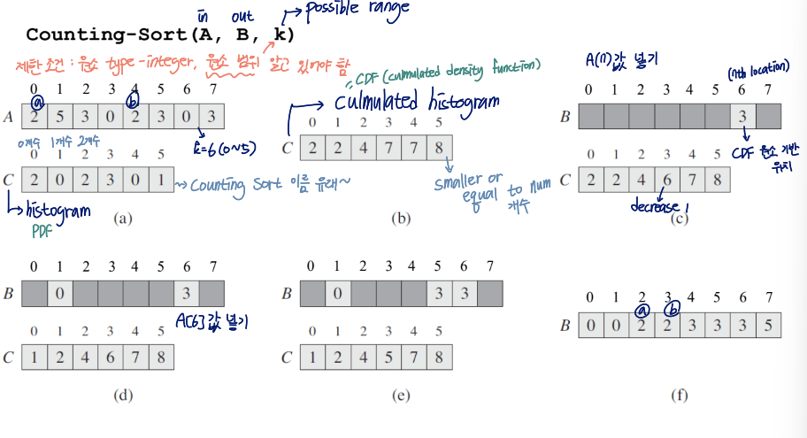
이게,,,어떻게 설명을 해야될지 모르겠네...그냥 코드 보면 이해 되니까 코드 보기로 하잡..

C code

//A: input, B: output, k: possible range(원소 범위)
void counting_sort(A, B, k){
	for(int i=0; i<k; i++){
    	C[i] = 0;
    }
    for(int j=0; j<n; j++){	 //n: size of A
    	C[A[j]] += 1; 		//histogram(=PDF)
    }
    for(int i=1; i<k; i++){
    	C[i] += C[i-1];		//cumulated histogram(CDF)
    }
    for(int j=n-1; j>=0; j++){
    	B[C[A[j]]-1] = A[j];
        C[A[j]] -= 1;
    }
}

for문 중 i를 사용하는 것들:takes O(k) time
for문 중 j를 사용하는 것들:takes O(n) time

Time Complexity of Counting Sort

Total time: O(n+k)

• usually, k=O(n) → k is ignorable
  → counting sort runs in O(n) time
• there are no comparisons at all

k가 n보다 much smaller한 경우(ex.n=10000, k=500)에 counting sort에서 advantage를 얻을 수 있음
→ n=3, k=0~20101인 경우는 memory wasting이 심해서 meaningless

this algorithm is stable
numbers with the same value appear in the output array in the same order as in the input array

Radix Sort

k가 큰 경우, counting sort에서의 benefit을 챙기며 sort하고 싶을 때를 위한 아이디어

Key idea

sort the number for each digit

• Sorting order does matter
• Most significant digit(MSD) vs. Least significant digit(LSD)
• Sort the least significant digit(LSD) first

counting sort가 stable sort라서 이것도 statble sort

Example

오른쪽일수록 less significant → 맨오른쪽부터 sort

Time Complexity of Radix Sort

Total compelxity

• for n numbers with d digits, assume each pass ranged 0 to k
• time complexity of each pass: O(n+k)
• total time: O(d(n+k))
• when d is constant and k=O(n), takes O(n) time

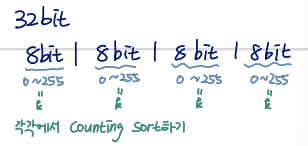
Example

sort 1 milion 64-bit numbers

• treat the data as four-digit radix
• each digit ranges 0~2^16-1

→ O(4(n+2^16))
typical comparison-based sort보다 훨씬 빠름

Radix Sort using Queue

Procedure

1. set a set of queues for range
2. execute 'eunqueue' and 'dequeue'
3. iterate 1-2 for each pass(e.g. digit1 -> digit2)
   

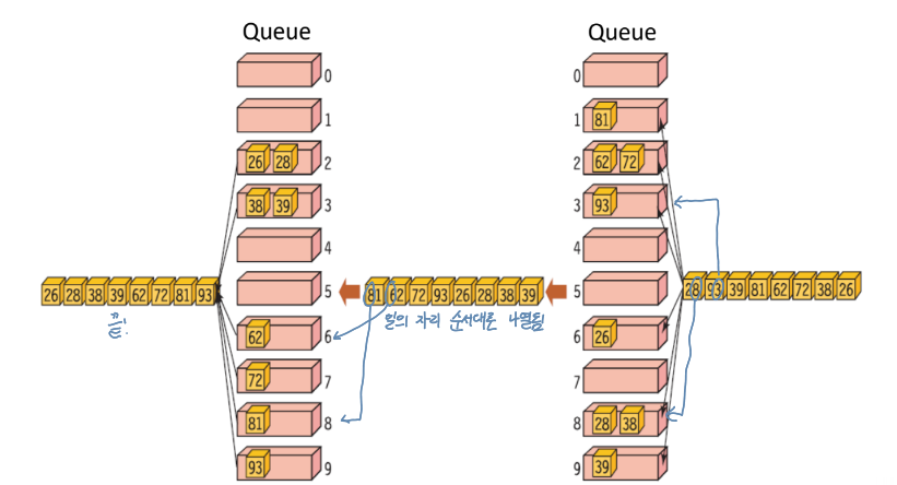
C code

#define BUCKETS 10
#define DIGITS 4

void radix_sort(int list[], int n){
	int i, b, d, factor = 1;
    QueueType queues[BUCKETS];
    
    for(b=0; b<BUCKETS; b++) init(&queues[b]);
    
    for(d=0; d<DIGITS; d++){
    	for(i=0; i<n; i++){
        	enqueue(&queues[(list[i]/factor) % BUCKETS], list[i]);
        }
        for(b=i=0; b<BUCKETS; b++){
        	while(!is_empty(&queues[b])){
            	list[i++] = dequeue(&queues[b]);
            }
        }
        factor*=BUCKETS;
    }
}

근데 queue보다 histogram 사용이 메모리를 적게 사용해서 histogram 사용해서 radix sort를 하는 것이 더 좋음

Runtime Measure Example

	Runtime(sec)
Insert sort	7.438
Selection sort	10.842
Bubble sort	22.894
Shell sort	0.056
Quick sort	0.014
Heap sort	0.034
Merge sort	0.026

생각보다 runtime 차이가 엄청나다!
따라서 sort 사용할 때 time complexity 유의하면서 방법 선택하는 게 좋음!