머신러닝-4단계(튜닝 : Random Search/Grid Search)

1. 튜닝 개념

• 1) KNN 알고리즘의 경우, n_neighbors 값의 설정에 따라 모델의 성능이 달라진다.

---

• 2) Decision tree/Random Forest/XGBoost/LGB의 경우, max_depth 값의 설정에 따라 모델의 성능이 달라진다.

---

• 3) cross_var_score를 사용하여 성능 예측을 통해, 사용할 알고리즘을 선택한 경우,

  • 해당 알고리즘의 매개변수를 어떻게 설정할 것인지, 결정할 때 튜닝을 사용한다.

  ---

• 4) 튜닝의 방법은 2가지가 있다.

  • Grid Search : parameter에서 설정한 범위를 전부 탐색, n_iter 설정 x

  • Random Search : parameter에서 설정한 범위에서 n_iter=3일 때, 3개만 탐색

---

• 5) 튜닝 횟수는 (범위 * cv값)임으로 Grid 방법일 때, 많은 시간이 소요된다.

---

• 6 함수 불러오기 : 뒤에 CV가 따라 온다.

from sklearn.model_selection import RandomizedSearchCV
from sklearn.model_selection import GridSearchCV

---

• 7) 튜닝 수행 후, 확인해야 하는 값

1) model.cv_results_['mean_test_score']
2) model.best_params_
3) model.best_score_
4) model.best_estimator_.feature_importances_

2. ex)

• 데이터 분리 완료했다고 가정.

---

1. 성능 예측

# 불러오기
from sklearn.tree import DecisionTreeRegressor
from sklearn.model_selection import cross_var_score, RandomizedSearchCV
from sklear.metrics import mean_absolute_error, r2_score

# 선언하기
model = DecisionTreeRegressor(random_state=1)

# 성능예측
cv_score = cross_var_score(model, x_train, y_train, cv=5)

# 결과확인
print(cv_score)
print('평균 :', cv_score.mean())
<출력>
[0.65873754 0.49225288 0.78163071 0.80327749 0.82834327]
평균 : 0.7128483767547819
------------------------------------------------------------------------
(회귀 유형에 사용되는 알고리즘 다 봐야되지만, Decision Tree만 확인)
------------------------------------------------------------------------

---

2. 모델 튜닝

# 파라미터 선언
param = {'max_depth' : range(1, 51)}

# 기본모델 선언
model_dt = DecisionTreeRegresor(random_state=1)

# Random Search 선언
model = RandomizedSearchCV(model_dt,        # 기본 모델
                          param,            # 파라미터 범위
                          cv=5,             # k-fold 개수
                          n_iter=20,)       # 랜덤하게 선택할 파라미터(조합) 개수 
                          					# Grid Search인 경우에는 n_iter 설정하지 않는다.
# 학습하기
model.fit(x_train, y_train)    			    # 여기서 시간이 많이 걸림.

# 결과확인
1. print(model.cv_results_['mean_test_score']
2. print(model.best_params_)                     # 최적 파라미터
3. print(model.best_score_)                      # 최고 성능
<출력>
================================================================================
[0.7003743  0.71284838 0.70520623 0.71284838 0.71284838 0.71284838
 0.71284838 0.71284838 0.71284838 0.71284838 0.71284838 0.71284838
 0.71090334 0.71284838 0.71284838 0.71278394 0.71284838 0.74748839
 0.71284838 0.71332444]
--------------------------------------------------------------------------------
최적파라미터: {'max_depth': 6}
--------------------------------------------------------------------------------
최고성능: 0.7474883885080482    # 그냥 성능예측 했을 때 : 0.7128483767547819
================================================================================

---

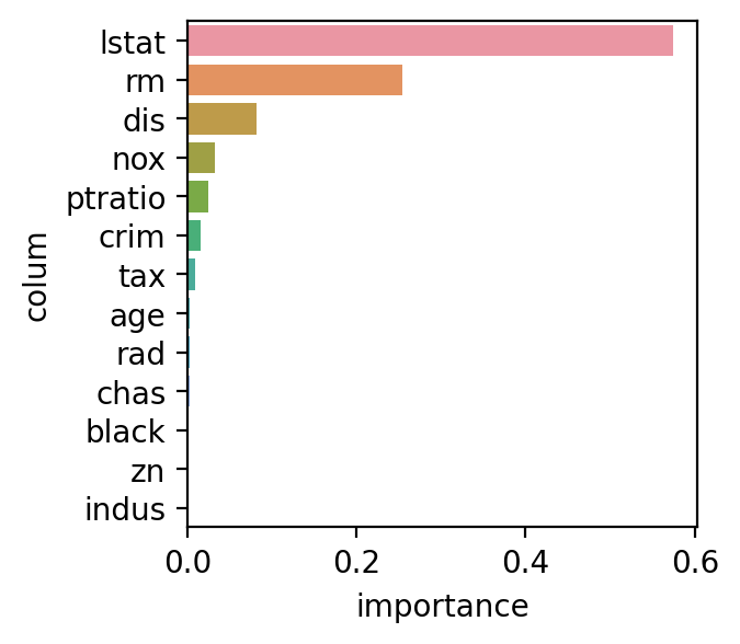
3. 변수 중요도 시각화

df = pd.DataFrame()
df['colum'] = list(x)
df['importance'] = model.best_estimator_.feature_importances_
df.sort_values(by = 'importance', ascending = False, inplace = True)

sns.barplot(x = 'importance', y = 'colum', data = df)
<출력>

---

4. 성능평가

y_pred = model.fit(x_train, y_train)

print(mean_absolute_error(y_test, y_pred))
print(r2_score(y_test, y_pred))
<출력>
MAE: 2.763239793643037
R2-Score: 0.8477248406093285