7. Clustering (2)

1. Basic Clustering Methods: Hierarchical Methods

1.1 Why Hierarchical Clustering?

Multiple levels of granularity

• In many real scenarios, data naturally forms groups at different levels
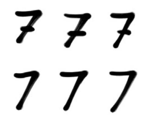
• E.g., organization charts or handwriting styles

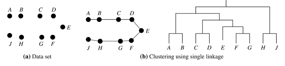
Dendrogram

• The result is a tree structure that supports many possible clusterings by "cutting" the tree at different heights

단순히 k개로 나누기가 아니라 덴드로그램이라는 트리 구조를 만든다. 높이에 따라 자르면 다양한 단계의 군집을 얻을 수 있다.

1.2 Two Viewpoints of Hierarchies

1. Representational Tool

• Do not assume the data has an inherent hierarchical structure
• Mainly used to summarize and visualize the data
• E.g., in HR analytics, a hierarchy (executives $\rightarrow$ managers $\rightarrow$ staff) makes it easy to compute summaries like average salary per level

데이터가 원래 그렇게 생겨서가 아니라, 계층적으로 분류해서 보는 것이 유용하기 때문에 계층적 군집화를 쓴다.

2. Underlying Data Structure

• Assume there is an intrinsic hierarchical structure and try to recover it
• E.g.,
  • Evolutionary biology: clustering organisms to recover phylogenetic trees
  • Strategic games: clustering game configurations to reveal hierarchical strategy patterns

In both cases, the hierarchical representation lets us reason about data at multiple resolutions

---

2. Agglomerative Hierarchical Clustering

2.1 Agglomerative (bottom-up)

Hierarchical clustering methods differ in how they build the tree: Bottom-up vs. Top-down

• Start with each object as its own cluster
  • 데이터가 n개 있다면, 처음에는 n개의 군집이 존재
• Iterative merge clusters until objects are in a single cluster
  • Or until some stopping condition is met
• At each step:
  • Compute pairwise distances (or similarities) between existing clusters
  • Find the two closest clusters
  • Merge them into a new cluster
• The final single cluster at the top is the root of the hierachy
• If there are $n$ objects, the methods requires at most $n-1$ merges

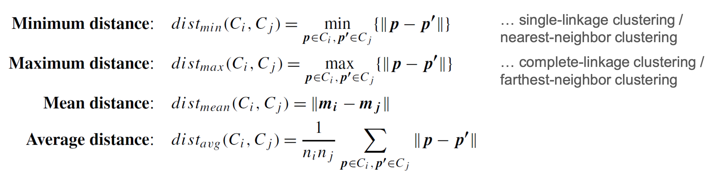
2.2 Linkage Measures

• Suppose $C_i$ and $C_j$ are two clusters, $p$ and $p'$ are objects, $m_i$ is the mean cluster $C_i$, and $n_i$ is the number of objects in $C_i$
• The most common linkage measure are the following

Example

• Cluster A: A1 = (1, 1), A2 = (2, 1) / Cluster B: B1 = (5, 1), B2 = (6, 1)
• All pairwise distances
  • Single distances = 3
  • Complete distances = 5
  • Mean distance = 4
  • Average distance = 4

2.3 Interpretation

1. Single linkage

• Discover clusters based on local proximity
• May connect objects through a chain of nearby points
• Even when the overall cluster shape is elongated or loose

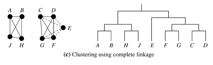
2. Complete linkage

• Discover clusters based on global closeness
• Prefers compact and tight clusters
• Because it penalizes large internal spread

3. Mean distance

• Simple and efficient because it summarizes each cluster with its centroid
• Mainly suitable when cluster means are meaningful and well-defined
• E.g., spherical cluster vs. non-convex or curved cluster

주로 구형 군집에 적합하며 볼록하지 않거나 휘어진 형태에는 취약할 수 있다.

4. Average distance

• Provides a compromise between minimum and maximum linkage
• Relies on all cross-cluster pairwise distances
• It is often more balanced

2.4 Strenthes and Weaknesses

Sensitive to outliers

• In single linkage
  • One unusual point may act as a bridge and connect two otherwise separate clusters
• In complete linkage
  • One distant outlier can make two otherwise similar clusters appear very far apart
• Mean distance and average distance are often considered more stable compromises

Mean distance vs. Average distance

• Mean distance
  • Usually the simplest to compute because it compares only the cluster means
  • This makes it computationally attractive when the data are numerical
• Average distance
  • More flexible because it does not need a cluster centroid to be defined
  • Categorical data or mixed-type data, as long as a distance function

---

3. Connecting to Partitioning Methods

3.1 Why is there a connection?

Cluster compactness

• Agglomerative hierarchical clustering and partitioning methods may seem different
• But they are related through the idea of cluster compactness

Sum of Squared Errors

• Partitioning methods evaluate a clustering by using the SSE
• Which measures how tightly the objects are grouped around their cluster means

Starting point

• If a dataset contains $n$ points, then a partition into $n$ clusters means that each point forms its own cluster
• This is exactly the starting point of agglomerative hierarchical clustering, where the algorithm begins with singleton clusters and then repeatedly merges them

Natural heuristic for merging

• Which two clusters should be merged next?
• A natural heuristic is to merge the pair that causes the smallest increase in SSE, because this keeps the clustering as compact as possible

3.2 Ward’s Method

1. Definition

• Measures similarity by asking how much the total within-cluster SSE would increase if two clusters were merged
• Selection rule
  • The pair for which the within-cluster SSE increases the least after merging is regarded as the most similar

2. Mathematical Criterion

$W(C_i, C_j) = \sum_{\mathbf{x} \in C_i \cup C_j} \|\mathbf{x} - m_{(ij)}\|^2 - \sum_{\mathbf{x} \in C_i} \|\mathbf{x} - m_i\|^2 - \sum_{\mathbf{x} \in C_j} \|\mathbf{x} - m_j\|^2$

• 병합 후의 SSE에서 병합 전 군집의 SSE 합을 뺀 값
• 두 군집을 하나로 합쳤을 때 발생하는 SSE의 순수 증가량을 구하는 식

$W(C_i, C_j) = \frac{n_i n_j}{n_i + n_j} \|m_i - m_j\|^2$

• 두 군집의 크기와 중심점 간의 거리만을 이용하여 동일한 결과를 얻을 수 있도록 유도된 식
• Cluster size $\times$ distance between centriods

3. Interpretation and Strategy

• Smallest possible increase in within-cluster variance
• As a greedy strategy, it tries to preserve compact and low-variance clusters
• Tend to merge clusters whose centriod are close, while also accouting for their sizes

---

4. Divisive Hierarchical Clustering

4.1 Divise (top-down)

• Start with all objects in one cluster (the root)
• Iteratively split clusters into smaller subclusters
• Recursively apply splitting to the resulting subclusters
• Stop when:
  • Each cluster has just one object, or
  • Clusters at the lowest level are sufficiently coherent (objects in each cluster are very similar)

4.2 Basic Ideas & Three Key Questions

---

4. BIRCH

4.1 Motivation and Core Idea

4.2 Clustering Feature

4.3 Two Phases of BIRCH

4.4 Effectiveness and Limitations