7. Clustering (1)

1. Cluster Anaysis

1.1 What is Cluster Anaysis

Definition

• Cluster analysis partitions a set of data objects into subsets called clusters
• Objects within a cluster are similar to each other, while objects in different clusters are dissimilar

Unsupervised Learning

• No class labels are given; groups are discovered automatically from the data
• Different clustering methods
  • or the same method with dirrerent parameters or initializations
  • can produce different clusterings on the same data set

Purpose

• To discover previously unknown groups or structures in the data
• Each cluster can be treated as an implicit class that later be interpreted and labeled by humans

1.2 Clustering Application

Business Intelligence

• Grouping customers into segments with similar characteristics to support targeted marketing
• E.g., scenario, client type, required expertise, duration, and size

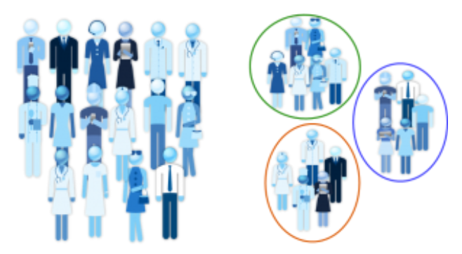
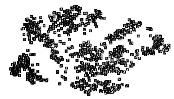
Image Pattern Recognition

• Discover clusters or "subclasses" in photos
• Clustering uses visual features to group similar images

Outler Detection

• Points that are far from any cluster can be treated as outliers, which may correspond to rate but important events
• E.g., credit card fraud, abnormal e-commerce behavior

1.3 Requirements

A pratical clustering algorithm must satisfy several requirements beyoung simple "distance-based grouping"

• Real data
  • Large-scale
  • Noisy and incomplete
  • High-dimensional
  • Heterogeneous

1. Scalability

• Modern applications handle millions to billions of objects
• Time and memory complexity should scale near-linearly in $N$

2. Arbitrary-shape cluster discovery

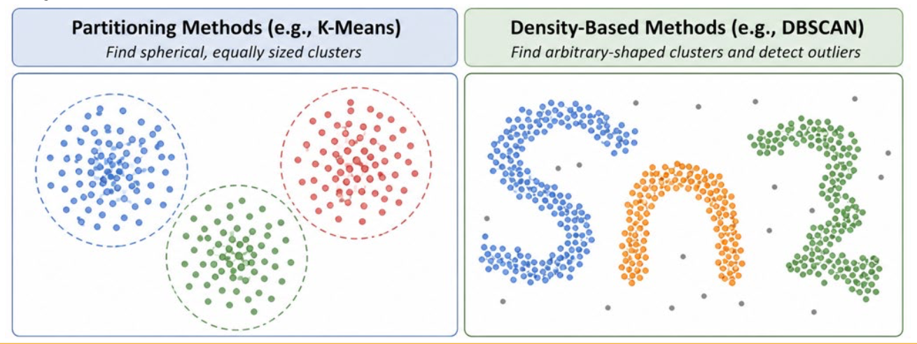
• Distance-based methods tend to favor spherical, similar-sized clusters
• Must detect non-convex and irregularly shaped clusters

실제 생활의 데이터는 대부분 구형이 아니며 불규칙한 모양을 가진다.

3. Robustness to noise & outliers

• Real-world data contain measurement errors, missing values, and outliers
• Should tolerate noise and explicitly identify or minimize the influence of outliers

4. High-dimensional data handling

• High-dimensional data suffers from the curse of dimensionality — sparse, skewed, and less meaningful distances
• Address via dimensionality reduction, feature selection, or projection-based strategies

5. Limited domain knowledge dependency

• Parameters like $k$ or density thresholds are hard to set and highly sensitive
• Fewer, interpretable parameters that can be tuned in a data-driven way are preferred

6. Interpretability and usability

• Cluster results should map to clear semantic concepts understandable by domain experts
• Feature selection, data representation, and algorithm choice should reflect the end application

---

2. Basic Clustering Methods

2.1 Partitioning Methods

• Divides a data set of $n$ objects into $k$ groups
  • Typically, $k \le n$ and is chosen as a relatively small number

Mechanism

• Most partitioning methods are distance-based and start with an initial clustering, then iteratively relocate to improve cluster quality

Goal

• In the same cluster close to one another
• While making objects in different clusters far apart

Characteristics

1. Basic setting = hard clustering
   • Each object belongs to exactly one cluster
2. Fuzzy partitioning = soft clustering
   • An object may belong to multiple clusters with different probabilities (between 0 and 1)
3. Global optimum is computationally expensive to find
   • Practical methods usually rely on heuristics such as k-means and k-medoids
   • These often work well for spherical clusters in small- to medium-sized data sets

어떤 기준점으로부터의 거리를 따지는 기하학적 특성상(유클리드 거리) 구형 군집이라는 틀에 갇히기 쉽다. 다만 그 기준점이 반드시 평균일 필요는 없다.

2.2 Hierarchical Methods

• Builds a hierarchical decomposition of the data rather than a single flat partition

Mechanism

• Agglomerative(bottom-up)
  • Start with each object as its own cluster and repeatedly merge nearby clusters
• Divisive(top-down)
  • Start with all objects in one cluster and repeatedly split clusters into smaller ones

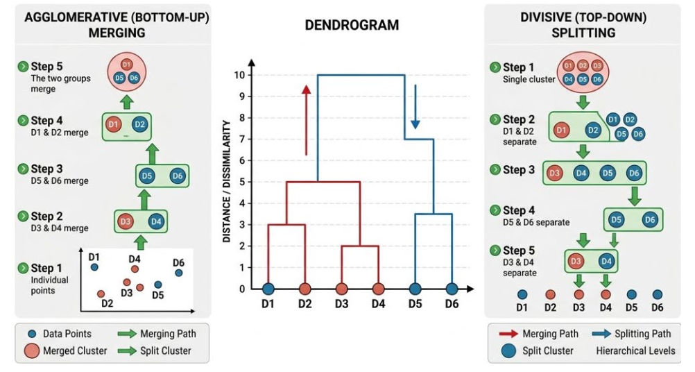
하나의 데이터가 작은 군집(자식)에서 시작해서 큰 군집(부모)로 계속 확장되어가는 구조를 가지게 된다.

Characteristics

1. Can be based on distance, density, or continuity
   • Can also be extended to subspace clustering
2. A merge or split decision is usually not undone $\rightarrow$ 결정의 비가역성

2.3 Density-based Methods

• Define cluster as regions where the local density of points is high enough

Mechanism

• Grow a cluster as long as the neighborhood of a point contains at least a minimum number of nearby points within a specified radius

특정 반경 내 최소 포인트 수가 모이지 않는 경우, 해당 포인트는 노이즈 또는 이상치로 처리된다. 반면, k-means는 아무리 멀리 떨어진 데이터라도 어떻게든 가장 가까운 중심점에 할당하여 군집의 일부를 포함시키려 하기 때문에 결과가 왜곡된다.

Characteristics

• Useful because they can discover cluster of arbitrary shape
• Natually identify noise and outliers

중심점으로부터의 거리에 얽매이지 않고 밀도를 따라 군집을 형성하기 때문에 임의의 모양을 잘 찾아내고 최소 밀도라는 문턱값이 존재하여 노이즈를 식별하는 데에 유리하다.

2.4 Grid-based Methods

• Quantizes the data space into a finite number of cells and then performs clustering on the grid rather than directly on all objects

Mechanism

• Dense cells are treated as components of clusters, and neighboring dense cells can be combined to form larger clusters

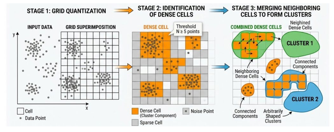
Characteristics

1. High efficiency
   • The processing cost depends mainly on the number of grid cells, not directly on the number of data objects
2. Useful for very large spatial data sets, and they can also be combined with hierarchical or subspace clustering ideas

일반적인 군집화는 수백만 개의 데이터 객체를 대조하여 연산 처리 비용이 데이터 객체의 총 개수에 의존한다. 그리드 방법은 데이터 공간을 유한한 수의 셀로 양자화한 뒤, 그리드 위에서 군집화를 수행하여 설정한 그리드 셀의 수에 의존한다.

---

3. K-means

3.1 Intuition

Partitioning clustering: basic idea

• Partitioning is the simplest and most fundamental form of cluster analysis
• Given a set of objects, we divide them into several exclusive groups (clusters)
• Each cluster is represented by a representative (e.g., centroid), and each object is assigned to the cluster whose representative it is closest to

Problem setup

• Input: data $D$ with $n$ objects and a desired number of cluster $k (k \le n)$
• Goal: partition $D$ into $k$ clusters $C_1, C_2, ..., C_k$, each non-empty and mutually exclusive
• Optimization
  • Intra-cluster similarity is high (objects within a cluster are similar)
  • Inter-cluster similarity is low (clusters are well separated)

• How do we choose the representatives of clusters (centroids/medoids)?
• How do we measure distance or similarity between objects and between objects and representatives?

3.2 Centroid-Based Partitioning

Centroid-based view

• k-means is a centroid-based partitioning algorithm for objects in Euclidean space
• Each cluster $C_i$ has a centroid, $c_i$, typically defined as the mean of the points in $C_i$
• The quality of a clustering is measured by the within-cluster sum of squared errors

$E = \displaystyle \sum^k_{i=1} \sum_{p \in C_i} dist(p, c_i)^2$

• Where dist is usually Euclidean distance
• The task is to find a partition that minimizes $E$ (compact and well-separated clusters)

Why do we need heuristics?

• Minimizing SSE exactly is computationally hard (NP-hard even for $k = 2$)
  • Because the number of possible partitions grows exponentially with $n$
• Therefore, practical algorithms use greedy/iterative heuristics to approach a good(local) optimum instead of the global optimum

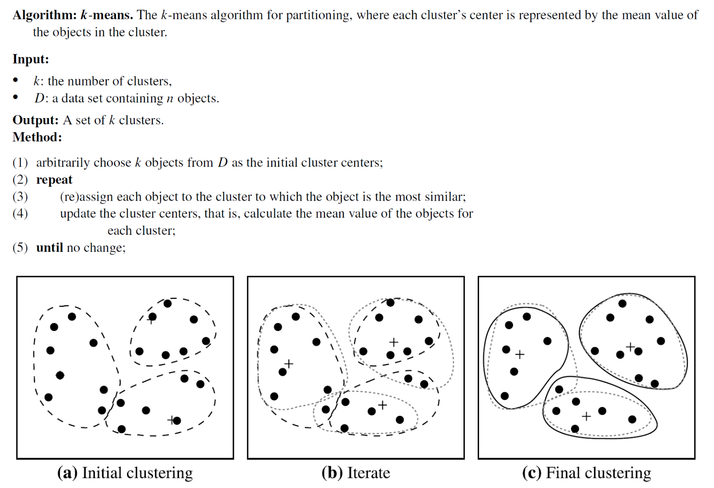
Basic k-means procedure

• Randomly choose $k$ objects as initial centroids
• Assignment step: assign each object to the cluster with the nearest centroid
• Update step: recompute each centroid as the mean of its assigned objects
• Repeat steps until cluster assignments no longer change (convergence)

Time complexity and practicality

• Time complexity: $O(nkt)$
  • $n$: number of objects, $k$: clusters, $t$: iterations until convergence (usually $t << n$)
• Scales linealy in $n$ and works well for large data sets with moderate dimensions

3.3 Pros & Cons

Advantages

• Conceptually intuitive and easy to implement
• Widely available in statistical, data mining, and ML toolkits
• Guaranteed to converge to some local optimum
• Supports “warm start” (user-specified initial centroids)

Limitations

• Requires the user to specify $k$ in advance
• Results are sensitive to initial centroids; require multiple runs with different initializations
• Has difficulty with clusters of very different sizes/densities and is sensitive to outliers
• Performance may degrades on high-dimensional data

3.4 Example: Clustering by k-menas partitioniong

Example

• Data points in 1D: {1, 2, 3, 8, 9, 10, 25}
• Intuitively, we would cluster {1, 2, 3} and {8, 9, 10}, treating 25 as an outlier
• Using k-means with $k$ = 2 and SSE objective
  • Partition A: {{1, 2, 3}, {8, 9, 10, 25}} $\rightarrow$ means: 2 and 13 $\rightarrow$ SSE = 196
  • Partition B: {{1, 2, 3, 8}, {9, 10, 25}} $\rightarrow$ means:3.5 and 14.67 $\rightarrow$ SSE $\approx$ 189.67
• k-means therefore chooses partition $B$ and separates 8 from 9 and 10
  • Because of the influence of the outlier 25
  • The second centroid (14.67) is also far from all its member points, so it is a poor representative of the cluster

Key drawback

• k-means is highly sensitive to outliers; a few extreme values can distort cluster assignments and produce centroids that do not correspond well to any actual data points

출처:
Hierarchical Cluster Analysis: https://uc-r.github.io/hc_clustering