📦 Schedulability analysis of global scheduling algorithms on multiprocessor platforms

이게 가능하도록 해준 Marp에게 무한한 감사를!

1. Introduction

• In this paper, the problem of preemptively scheduling a real-time task set on a symmetric multiprocessor (SMP) system consisting of $m$ processors is addressed.
• Can be solved in two different ways
  • by partitioning tasks to processors
  • with a global scheduler
• Semi-partitioned scheduling : limits the number of processors among which a task can migrate
• Pfair scheduling : at each quantum the scheduler allocates tasks to processors.
  • Known to be optimal when deadlines = periods
  • Disadvantages: quantum synchronize, context switching overhead, complex
  • job-level dynamic

---

1.1 Contribution

1. General conditions that are valid for any work-conserving scheduling algorithm and constrained deadline task sets
   • Fixed Priority (FP)
   • The Earliest Deadline First (EDF).
2. The main weak points of feasibility tests and further refinement on the computation of the interference a task can be subject to.
3. Finally, an extensive set of synthetic experiments is presented to show the improved performances of our analysis.

---

2. System Model

Symbols

• A task $\tau_k$ is a sequence of jobs $J^j_k$
• $J^j_k(r^j_k,d^j_k,c^j_k,f^j_k)$: arrival time, deadline, computation time, finishing time
• $\tau_k = (C_k, D_k, T_k) \in \tau$
  • $C_k$: worst-case computation time, $C_k \ge c_k^j$
  • $D_k$: relative deadline, $d^j_k = r^j_k + D_k$
  • $T_k$: minimum interarrival time, $r^j_k \ge r^{(j-1)}_k + T_k$
• constrained deadline (implicit deadline): $D_k \le T_k$ ($D_k = T_k$)
• utilization: $U_k = \frac{C_k}{T_k}$, density("worst-case" request): $\lambda_k = \frac{C_k}{D_k}$
• $U_{\max} = \displaystyle{\max}_k U_k$, $\lambda_{\max} = \displaystyle{\max}_k \lambda_k$, $U_{tot} = \displaystyle\sum_{\tau_k \in \tau} U_k$, $\lambda_{tot} = \displaystyle\sum_{\tau_k \in \tau} \lambda_k$

---

Notation

• $(x)_0 = {\max}(0, x)$

Definition

• Work-conserving : A scheduling algorithm is work-conserving if there are no idle processors when a ready task is waiting for execution.

---

2.1 Workload and Interference

• Workload $W_k(a, b)$ : the amount of time task $\tau_k$ executes during interval $[a, b)$
• Interference $I_k(a, b)$ : the cumulative length of all intervals in which $\tau_k$ is ready to execute, but it cannot execute due to higher priority jobs.
  • $I_{i,k}(a, b)$ : the cumulative length of all intervals in which $\tau_k$ is ready to execute, and $\tau_i$ is executing while $\tau_k$ is not.

---

2.2 Time division

• Time-instants and interval lengths are often modeled using real numbers, in a real implemented system time is not infinitely divisible.
• The times of event occurrences and durations between them cannot be determined more precisely than one tick of the system clock.
• $t$ (non-negative integer value) represents the entire interval $[t, t + 1)$

---

3. Summary of existing results

Theorem 1.
A task set $\tau$ composed by periodic and sporadic tasks with implicit deadlines is EDF-schedulable upon a SMP composed by $m$ processors with unitary capacity, if

$U_{tot} \le m(1 −U_{\max}) + U_{\max} \tag{2}$

When deadlines can differ from periods?

---

Theorem 2.
A set of jobs $I$ that is feasible on some uniform multiprocessor platform $\pi$ with cumulative computing capacity $S_\pi$, and in which the fastest processor has speed $s_\pi < 1$, is schedulable with EDF on a SMP $\pi$ composed by m processors with unit capacity, if

$m \ge \frac{S_\pi-s_\pi}{1-s_\pi}$

• $i$th processor works for $t$ time units $\rightarrow$ $s_i \times t$ execution units.
• Theorem 2 assumes an arbitrary collection of jobs.
• The next lemma states a feasibility result that instead applies to periodic and sporadic task sets.

---

Lemma 1
A task system $\tau$ composed by periodic and sporadic tasks with constrained deadlines is feasible on a uniform multiprocessor platform $\pi$ which has $S_\pi = \lambda_{tot}$ and $s_\pi = \lambda_{{\max}}$

Proof

• An arbitrary task set $\tau$ with n tasks can always be scheduled on a uniform multiprocessor platform $\pi$ composed by n processors, that for each task $\tau_i$ has a corresponding processor with computing capacity $s_i = \frac{C_i}{D_i}$.
• This can be done with an algorithm that allocates each task to the associated processor.
• The sum of the computing capacities of all processors and the computing capacity of the fastest processor of the platform π are therefore equal to $\lambda_{tot}$ and $\lambda_{\max}$ respectively. $\blacksquare$

---

• By combining Lemma 1 with Theorem 2, it is possible to formulate a sufficient scheduling condition.

Theorem 3 GFB
A task set $\tau$ composed by both periodic and sporadic tasks with constrained deadlines is EDF-schedulable upon a SMP composed by $m$ processors with unitary capacity, if

$\lambda_{tot} \le m(1 − \lambda_{\max}) + \lambda_{\max}. \tag{3}$

• If $\lambda_{\max}$ is large, RHS of Equation $(3)$ remains small.
• This is due to a DHall's Effect

---

How to overcome DHall's Effect

1. EDF$^k$
   • Assign the highest priority to the k the heaviest tasks.
   • Schedule the remaining ones with EDF.
   • Schedulability test : Apply GFB to a subsystem composed by the $(n−k)$ EDF-scheduled tasks on $(m−k)$ processors.
2. EDF-US
   • Assign the highest priority to the tasks having utilization larger than given threshold.
   • Allows the utilization bound of $\frac{m+1}{2}$ when threshold of $\frac 1 2$ used.

---

• Baker's idea is based on the consideration that if a job $J^j_k$ of a task $\tau_k$ misses its deadline $d^j_k$.
• It means the load in problem window (an interval $[r^j_k, d^j_k)$) is at least $m(1-\lambda_k) + \lambda_k$
• If it's possible to show for every $J^j_k$, the schedulability is guaranteed.

---

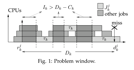
Carry-in

• The interference of any task $\tau_i$ on task $\tau_k$ in interval $[r^j_k, d^j_k)$ may include one job of $\tau_i$ with arrival before $r^j_k$ and deadline in $[r^j_k, d^j_k)$.
• The contribution of this job to the interference is called carry-in.

Sufficient schedulability condition

• Enlarge $[r^j_k, d^j_k)$ to $[a, d^j_k)$ : busy window
  • the largest possible interval such that the load is still greater than $m(1-\lambda_k) + \lambda_k$
• By deriving an upper bound on the load produced in the busy window, a sufficient schedulability condition is obtained.

---

Rate-monotonic & Deadline-monotonic Algorithm

• Previous works proved that an implicit deadline task set can be successfully scheduled on $m$ processors if the total utilization is at most $m^2/(3m−2)$ and every task has individual utilization less than or equal to $m/(3m−2)$.
• Also showed RM-US[$m/(3m − 2)$] - that gives the highest priority to the tasks with utilization greater than $m/(3m−2)$ and schedules the other ones with RM - can also reach the utilization of $m^2/(3m−2)$.

---

Theorem 4
A set of periodic or sporadic tasks with constrained deadlines is schedulable with Deadline Monotonic priority assignment on $m \ge 2$ processors if $\lambda_{tot} \le \frac m 2 (1-\lambda_{\max}) + \lambda_{\max}$

• A corollary of Theorem 4 is that using a hybrid version of deadline monotonic - called
  DM-DS[$1/3$] that gives the highest priority to tasks with density higher than $1/3$.
• It's possible to schedule every constrained deadline task set with $\lambda_{tot} \le (m+1)/3$

---

4. Scheduling analysis

To clarify the methodology, we briefly describe the main steps that will be followed to derive the schedulability test.

1. Start by assuming that a job $J^j_k$ of task $\tau_k$ misses its deadline $d^j_k$

2. Based on this assumption, we give a schedulability condition that uses the interference $I_k$ that the job must suffer in interval $[r^j_k, d^j_k)$ for the deadline to be missed;

3. If we were able to precisely compute this interference in any interval, the schedulability test would simply consist in the condition derived at the preceding step, and it would be necessary and sufficient.

4. Therefore, we give an upper bound to the interference in the interval and derive a sufficient scheduling condition.

---

4.1 Interference time

Lemma 2
The interference that a task $\tau_i$ causes on a task $\tau_k$ in an interval $[a, b)$ is never greater than the workload of the task in the same interval:

$\forall i,k,a,b \;\;\;\; I_{i,k} \le W_i(a,b) \le b-a$

• Lemma 2 is obvious

Lemma 3
For a work-conserving scheduler, the following relation holds:

$I_k(a,b) = \frac{\sum_{i \ne k}I_{i,k}(a,b)}{m}$

---

Lemma 4

$I_k(a,b) \ge x \Leftrightarrow \displaystyle\sum_{i \ne k}\min(I_{i,k}(a,b), x) \ge mx$

Proof If

$\displaystyle\sum_{i \ne k}\min(I_{i,k}(a,b), x) \ge mx$, it follows that

$\begin{aligned} I_k(a,b) &= \sum_{i \ne k}\frac{I_{i,k}(a,b)}{m}\\ &\ge \sum_{i \ne k}\frac{\min(I_{i,k}(a,b), x)}{m}\\ &\ge \frac {mx} m = x \end{aligned}$

---

Proof Only If

Let $\xi$ be the number of tasks for which $I_k(a,b) \ge x$.
If $\xi > m$, then $\displaystyle\sum_{i \ne k}\min(I_{i,k}(a,b), x) \ge \xi x \ge mx$.
Otherwise, $(m-\xi) \ge 0$ and using Lemma 3 and Equation $(1)$,

$\begin{aligned} \displaystyle\sum_{i \ne k} \min(I_{i,k}(a,b),x) &= \xi x + \sum_{i:I_{i,k} < x} I_{i,k}(a,b) \\ &= \xi x + mI_k(a,b) - \sum_{i:I_{i,k} \ge x} I_{i,k}(a,b)\\ &\ge \xi x + mI_k(a,b)-\xi I_k(a,b) \\ &= \xi x + (m-\xi)I_k(a,b) \\ &\ge \xi x + (m-\xi)x \\ &= mx \end{aligned}$

---

• It is clear that, for a job to meet its deadline, $I_{k}(r^j_k, d^j_k) \le D_k − C_k$.
• Let's define the worst-case inference for task $\tau_k$ as:
  $\bar{I}_k = {\max}_j(I_{k}(r^j_k, d^j_k)) = I_{k}(r^{j*}_k, d^{j*}_k)$
  where $j∗$ is the job instance in which the total interference is maximal.
• To simplify the notation, also define:
  $\bar{I}_{i,k} = I_{i,k}(r^{j*}_k, d^{j*}_k)$

---

Theorem 5
A task set $\tau$ is schedulable on a multiprocessor composed by $m$ identical processors iff for each task $\tau_k$

$\sum_{i \ne k}\min(\bar{I}_{i,k}, D_k-C_k+1) < m(D_k-C_k+1) \tag{4}$

Proof If

If Equation $(4)$ is valid, from Lemma 4 we have $\bar{I}_k < (D_k-C_k+1)$.
Therefore, $J^{j*}_k$ will be interfered for at most $D_k-C_k$ time units. (integer time assumptions)
It means, every job of $\tau_k$ will complete after at most $D_k$ and $\tau_k$ is schedulable.

---

Proof Only If

If $\sum_{i \ne k}\min(\bar{I}_{i,k}, D_k-C_k+1) \ge m(D_k-C_k+1)$, then

$\begin{aligned} \bar{I}_k &= \frac{\sum_{i \ne k} \bar{I}_{i,k}}{m} \\ &\ge \frac{\sum_{i \ne k}\min(\bar{I}_{i,k}, D_k-C_k+1)}{m}\\ &\ge \frac{m(D_k-C_k+1)}{m}\\ &= D_k-C_k+1 \end{aligned}$

Hence, $\tau_k$ is not schedulable.

---

4.2 Workload

• Theorem 5 cannot be used to check if a task set is schedulable without knowing how to compute the interference terms $\bar{I}_{i,k}$’s.
• Unfortunately, we are not aware of any strategy that can be used to compute the worst-case interferences starting from given task parameters.
• To sidestep this problem, we will use an upper bound on the interference.
  • An upper bound on the interference $I_{i,k}$ is the workload $W_i(r^{j∗}_k , d^{j∗}_k)$
  • An upper bound on the workload? - Find densest possible packing of jobs!

---

To simplify the presentation,

• carry-in $\epsilon_k$ of $\tau_k$ in an interval $[a,b)$ : the amount of execution produced by a job of $\tau_k$ having release time before $a$ and deadline after $a$.
• carry-out $z_k$ of $\tau_k$ in an interval $[a,b)$ : the amount of execution produced by a job of $\tau_k$ having release time in $[a,b)$ and deadline after $b$.

There is at most one carry-in and one carry-out job.

We denote them, respectively, as $J^\epsilon_i$ and $J^z_i$

---

• Since a job $J^j_k$ can be executed only in $[r^j_k, d^j_k)$ and for at most $C_k$ time units,
• It is immediate to see that the depicted situation provides the highest possible amount of execution in interval $[a, b)$.

---

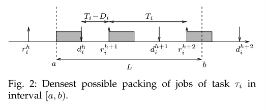
• The first job of $\tau_i$ after the carry-in, is released at time $a+C_i+T_i-D_i$.

• The next jobs released periodically every $T_i$ time units.

• Therefore, the number $N_i(L)$ of jobs of $\tau_i$ that contribute with an entire WCET to the workload in an interval of length $L$ is at most $\left\lfloor\frac{L-(C_i+T_i-D_i)}{T_i}\right\rfloor + 1$. So,

  $N_i(L) = \left\lfloor\frac{L+D_i-C_i)}{T_i}\right\rfloor \tag{5}$

• Continuously, the contribution of carried-out job can be bounded by $\min(C_i, L+D_i-C_i-N_i(L)T_i)$

• Now we can find the upper bound of workload:

  $\frak{W}\mathnormal{_i(L) = N_i(L)C_i+\min(C_i, L+D_i-C_i-N_i(L)T_i)} \tag{6}$

---

Theorem 6
A task set $\tau$ is schedulable with any work-conserving global scheduling policy on a multiprocessor platform composed by $m$ identical processors if for each task $\tau_k \in \tau$

$\sum_{i \ne k}\min(\frak{W}\mathnormal{(D_k), D_k-C_k+1) < m(D_k-C_k+1)} \tag{7}$

Proof
Equation $(6)$ is valid for any work-conserving scheduling algorithm.
Using Lemma 2, we then have

$\bar{I}_{i,k} = I_{i,k}(r^{j*}_k, r^{j*}_k+ D_k) \le W_i(r^{j*}_k, r^{j*}_k+ D_k) \le \frak{W}\mathnormal{(D_k)}$

Apply Theorem 5, using $\frak{W}\mathnormal{(D_k)}$ as an upper bound for $\bar{I}_{i,k}$.

---

4.3 Schedulability test for EDF

• There is no carried-out job can interfere with task $\tau_k$.
• We can consider the situation in which the carried-out job $J^z_i$ has its deadline at the end of the interval like Figure 3.

---

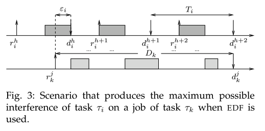
• There are $\left\lfloor \frac{D_k}{T_i} \right\rfloor$ jobs which contribute for an entire worst-case computation time.

• Instead, the first job contributes for $D_k-\left\lfloor \frac{D_k}{T_i} \right\rfloor T_i$ when this term is lower than $C_i$.

• We therefore obtain the following expression:

  $\bar{I}_{i,k} \le \left\lfloor \frac{D_k}{T_i} \right\rfloor C_i + \min \left( C_i, D_k - \left\lfloor \frac{D_k}{T_i} \right\rfloor T_i\right) = \frak{J}\mathnormal{_{i,k}} \tag{8}$

• A schedulability test for EDF immediately follows

Theorem 7
A task set $\tau$ is schedulable with global EDF on a multiprocessor platform composed by $m$ identical processors if for each task $\tau_k \in \tau$

$\sum_{i \ne k}\min(\frak{J}\mathnormal{_{i,k}, D_k-C_k+1) < m(D_k-C_k+1)} \tag{9}$

---

4.4 Schedulability test for FP

• It is still possible to use the general bound given by Equation $(6)$ that is valid for any work-conserving scheduling policy.
• The interference from tasks with lower priority is always null.
• The following theorem assumes tasks are ordered with decreasing priority.

Theorem 8
A task set $\tau$ is schedulable with fixed priority on a multiprocessor platform composed by $m$ identical processors if for each task $\tau_k \in \tau$

$\sum_{i < k}\min(\frak{W}\mathnormal{(D_k), D_k-C_k+1) < m(D_k-C_k+1)} \tag{10}$

---

5. Considerations

We must consider only the fraction of the workload that can actually interfere with task $\tau_k$.
When no task misses its deadline, this fraction is bounded by $D_k−C_k$

Example

Consider a task set $\tau$ composed by $\tau_1 = (1, 1, 1)$, $\tau_2 =(1, 10, 10)$, $\tau_3 =(1, 10, 10)$ and $\tau_4 =(1, 10, 10)$ to be scheduled with EDF on $m = 2$ processors. (It's schedulable.)

• When the deadlines of $\tau_1$ and $\tau_2$ coincide, a job of $\tau_2$ would need to be pushed forward for $D_2 − C_2 = 9$ time-units to interfere with $\tau_1$.
• But the maximum interference that $\tau_2$ is
  $I_2 \le \frac{\sum_{i \ne 2}I_{i,2}}{m} \le \frac{\sum_{i \ne 2}W_i(r^{j*}_2, d^{j*}_2)}{m} \le \frac {10 + 1 + 1} 2 = 6$

---

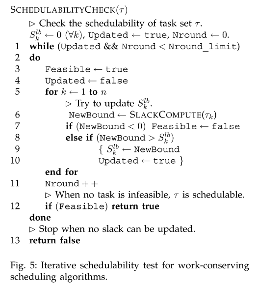
6. Iterative test

The lower the interference, the highest is the distance between the job finishing time $f^j_k$ and its deadline $d^j_k$.

• The slack $S^j_k$ of job $J^j_k:\;S^j_k = d^j_k-f^j_k$.
• The slack $S_k$ of task $\tau_k: S_k = \min_j(d^j_k-f^j_k)$

When $S_k>0$, the densest possible packing of jobs of $\tau_k$ will produce a lower workload in the considered interval.

---

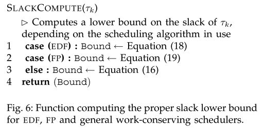
6.1 Iterative test for general scheduling algorithms

Theorem 9
The slack of a task $\tau_k$ scheduled on a multiprocessor platform composed by $m$ identical processors is given by

$S_k = D_k-C_k-\left\lfloor\frac{\sum_{i \ne k} \min(\bar{I}_{i,k}, D_k-C_k+1)}{m}\right\rfloor \tag{11}$

when Equation $(11)$ is positive.

---

Proof
When the RHS of Equation $(11)$ is positive, $\left\lfloor\frac{\sum_{i \ne k} \min(\bar{I}_{i,k}, D_k-C_k+1)}{m}\right\rfloor \le D_k-C_k$.
Applying Lemma 4, we have $\bar{I}_k < (D_k-C_k+1)$ and $\bar{I}_{i,k} \le \bar{I}_k < (D_k-C_k+1)$. Therefore,

$\min(\bar{I}_{i,k}, D_k-C_k+1) = \bar{I}_{i,k} \tag{12}$

Now, from the definition of slack,

$\begin{aligned} S_k &= \min_j(d^j_k - f^j_k) = d^{j*}_k - f^{j*}_k\\ &=(r^{j*}_k + D_k) - (r^{j*}_k+C_k+\bar{I}_k)\\ &= D_k-C_k-\bar{I}_k \end{aligned}$

Using Lemma 3 and Equation $(12)$,

$\begin{aligned} S_k &= D_k-C_k-\left\lfloor\bar{I}_k\right\rfloor \\&= D_k-C_k-\left\lfloor\frac{\sum_{i \ne k} \bar{I}_{i,k}}{m}\right\rfloor\\ &=D_k-C_k-\left\lfloor\frac{\sum_{i \ne k} \min(\bar{I}_{i,k}, D_k-C_k+1)}{m}\right\rfloor \end{aligned}$

---

Since we cannot compute $\bar{I}_{i,k}$ in a reasonable amount of time, we will use the upper bound on $\bar{I}_{i,k}$.

• We have $\frak{W}\mathnormal{_i(D_k) \ge \bar{I}_{i,k}}$

• A lower bound $S^{lb}_k$ on the slack of a task $\tau_k$ is then given by

  $S^{lb}_k = D_k-C_k-\left\lfloor\frac{\sum_{i \ne k} \min(\frak{W}\mathnormal{_i(D_k), D_k-C_k+1)}}{m}\right\rfloor \tag{13}$

Now, it's possible to give a tighter upper bound on the interference $\tau_i$.
Every job of $\tau_i$ will complete at least $S^{lb}_k$ time-units before its deadline if $S^{lb}_k$ is positive.

---

Let's override the expression of $\frak{W}\mathnormal{_i(L)}$ as follows:

Theorem 10
A lower bound on the slack of a task $\tau_k$ scheduled on a multiprocessor platform composed by $m$ identical processors is given by

$S^{lb}_k = D_k-C_k-\left\lfloor\frac{\sum_{i \ne k} \min(\frak{W}\mathnormal{_i(D_k, S^{lb}_i), D_k-C_k+1)}}{m}\right\rfloor \tag{16}$

when this term is positive.

---

 

• For every task in the task set, a lower bound value on the slack of the task is created and initially set to zero.
• Equation $(16)$ is then used to compute a new value of the slack lower bound of the first task, with $\frak{W}\mathnormal{_i(D_1, S^{lb}_i)}$ and $N_i(D_1, S^{lb}_i)$ given by Equation $(14)$ and $(15)$.
  • If the computed value is positive, the upper bound is accordingly updated.
  • If it is negative, the value is left to zero and the task is marked as temporarily not schedulable.
• The previous step is repeated for every task in the task set.
• If no task has been marked as temporarily not schedulable, the task set is declared schedulable.
• Otherwise, another round of slack updates is performed using the slack lower bounds derived at the previous cycle. If during a complete round no slack is updated, the iteration stops and the task set is declared not schedulable.

---

---

6.2 Iterative test for EDF

When a lower bound on the slack of $\tau_i$ is known, the upper bound on $\bar{I}_{i,k}$ given by Equation $(8)$ can be tightened.

---

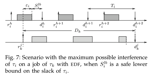
• The first job contributes for ${\max}\left(0, D_k-S^{lb}_k-\left\lfloor\frac{D_k}{T_i}T_i\right\rfloor\right)$ when this term is lower than $C_i$.
• This leads to following expression:
  $\bar{I}_{i,k} \le \left\lfloor \frac{D_k}{T_i} \right\rfloor C_i + \min \left( C_i, \left(D_k -S^{lb}_k- \left\lfloor \frac{D_k}{T_i} \right\rfloor T_i\right)_0\right) = \frak{J}\mathnormal{_{i,k}(S^{lb}_k)} \tag{17}$

Theorem 11
A lower bound on the slack of a task $\tau_k$ scheduled with EDF on a multiprocessor platform composed by $m$ identical processors is given by

$S^{lb}_k = D_k - C_k - \left\lfloor\frac 1 m \sum_{i \ne k} \min(\frak{J}\mathnormal{_{i,k}(S^{lb}_k), D_k-C_k+1)}\right\rfloor \tag{18}$

when this term is positive.

---

 
Assuming tasks are ordered with decreasing priority, next theorem follows.

Theorem 12
A lower bound on the slack of a task $\tau_k$ scheduled with fixed priority on a multiprocessor platform composed by $m$ identical processors is given by

$S^{lb}_k = D_k-C_k-\left\lfloor\frac{\sum_{i < k} \min(\frak{W}\mathnormal{_i(D_k, S^{lb}_i), D_k-C_k+1)}}{m}\right\rfloor \tag{19}$

when this term is positive.

However, there is an important difference from the EDF and the general case.

• When a task is found temporarily not schedulable during the first iteration, the test can immediately stop and return a false value.
• It means, we can choose $N\text{round\_limit}=1$ when the scheduler is FP

---

7. Experimental Results

We will consider the following schedulability algorithms for each case.

EDF

• Theorem 3 GFB, $O(n^3)$ test BAK
• Theorem 7 BCL EDF
• The iterative test when EDF is used. I-BCL EDF

FP - deadline monotonic

• Theorem 4 DB, $O(n^3)$ test BC
• Theorem 8 BCL FP
• The iterative test when FP is used.

General : BCL, I-BCL

---

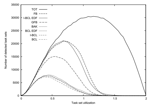
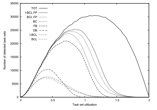
• Less than 1% of the generated task sets is found schedulable by an existing algorithm for EDF but not by I-BCL EDF.
• I-BCL FP outperforms even FB.

---

8. Computational Complexity

• Complexity of Theorems 6, 7, 8:
  $O(n^2)$: Each test involves $n$ inequalities with $n$ terms per inequality.

• Iterative Tests (Section 6):
  Complexity depends on the number of slack updates.

  $N\text{round\_limit} = \infty$:

  • Single iteration: $O(n^2)$
  • Total iterations: $O(nD_{{\max}})$
  • Overall complexity: $O(n^3D_{{\max}})$

  With finite $N\text{round\_limit}$:

  • $O(n^2N{\text{round\_limit}})$

---

Experimental Findings

Experiments with $N_{\text{round\_limit}} = 1, 2, 3, \infty$ in EDF case:

• $N\text{round\_limit} = 1$: Similar results to BCL EDF (Theorem 7).
• $N\text{round\_limit} = 2$: Significant increase in detected task sets.
• $N\text{round\_limit} = 3$: Detects almost all schedulable task sets as $N{\text{round\_limit}} = \infty$.

Optimal Trade-off:

• $N\text{round\_limit} = 3$ balances computational efficiency and performance.

---

9. Conclusions

Key Contributions:

• Developed schedulability analysis for real-time systems globally scheduled on identical multiprocessor platforms.
• Proposed sufficient schedulability tests with polynomial and pseudo-polynomial complexity.
• Iterative test detects the highest number of schedulable task sets compared to existing tests, with minimal missed sets.

Iterative Test Performance

• Iterative tests significantly increase the number of detected schedulable task sets.
• Only a small percentage of task sets are schedulable by existing tests but not by the iterative test.

---

EDF Limitations:

• EDF’s superiority in uniprocessor systems does not generalize to multiprocessors.
• Fixed Priority (FP) schedulers provide similar schedulability with lower implementation costs.

Fixed Priority (FP):

• I-BCL FP detects the most schedulable task sets among all existing FP-based algorithms.
• Combining simple FP schedulers with I-BCL FP ensures hard real-time constraints.