대회설명

-
대회의 목표는 와인의 퀄리티(quality)의 등급을 맞추는 것이다.
-
Feature X는
-
id : 식별 고유값
-
fixed acidity : 고정(비휘발성) 산도: 와인과 관련된 대부분의 산
-
volatile acidity : 휘발성 산도: 와인에 함유된 아세트산의 양. 너무 높으면 불쾌한 식초 맛이 날 수 있음
-
citric acid : 구연산: 소량으로 발견되며, 와인에 풍미를 더할 수 있음
-
residual sugar : 잔여 당분: 발효가 멈춘 후 남은 설탕의 양으로 1g/L 미만의 와인은 드물며 45g/L 이상의 와인은 단맛으로 간주함
-
chlorides : 염소화물: 와인의 염분량
-
free sulfur dioxide : 유리 이산화황: 미생물의 성장과 와인의 산화를 방지함
-
total sulfur dioxide : 총 이산화황: 저농도에서는 대부분 맛이 나지 않으나 50ppm 이상의 농도에서 맛에서 뚜렷하게 나타남
-
density : 밀도: 알코올 및 당 함량에 따라 변함
-
pH : 산성 또는 염기성 정도. 0(매우 산성) ~ 14(매우 염기성). 대부분의 와인은 pH 3-4 사이임
-
sulphates : 황산염: 이산화황 농도에 기여할 수 있는 와인 첨가제. 항균 및 항산화제로 작용
-
alcohol : 와인의 알코올 함량 백분율
-
type : 와인에 사용된 포도의 종류. Red(적포도주), White(백포도주)로 나뉨
-
y는
-
quality : 맛으로 평가된 와인의 품질
평가방법
- 평가는 Accuracy로 이루어진다.

1 Setting
1.1 Library Setting
import pandas as pd
import numpy as np
import matplotlib.pyplot as plt
import seaborn as sns
from matplotlib import patches
# seaborn setting
sns.set_theme(style='whitegrid')
sns.set_palette("twilight")1.2 Data Import
# 데이터 기본 path 설정
base_path = ".../data/"
# Training and Testing sets
train = pd.read_csv(base_path + "train.csv", encoding='cp949')
test = pd.read_csv(base_path + "test.csv")
## submission
submission = pd.read_csv(base_path + "sample_submission.csv")1.2.1 Training Set
train.head()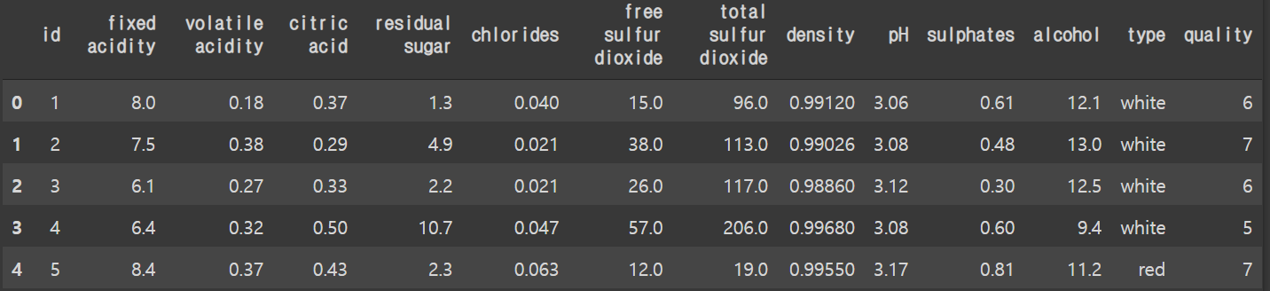
-
type의 경우 white 와 red로 나뉜 categorical 형식이다.
white를 0 red를 1로 변환시킨다.
whiteOrRed = {"white": 0, "red": 1}
train['type'] = train['type'].replace(whiteOrRed)
train.describe()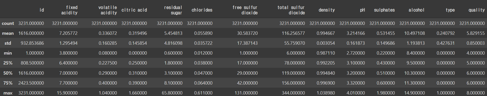
train.info()<class 'pandas.core.frame.DataFrame'>
RangeIndex: 3231 entries, 0 to 3230
Data columns (total 14 columns):
# Column Non-Null Count Dtype
--- ------ -------------- -----
0 id 3231 non-null int64
1 fixed acidity 3231 non-null float64
2 volatile acidity 3231 non-null float64
3 citric acid 3231 non-null float64
4 residual sugar 3231 non-null float64
5 chlorides 3231 non-null float64
6 free sulfur dioxide 3231 non-null float64
7 total sulfur dioxide 3231 non-null float64
8 density 3231 non-null float64
9 pH 3231 non-null float64
10 sulphates 3231 non-null float64
11 alcohol 3231 non-null float64
12 type 3231 non-null int64
13 quality 3231 non-null int64
dtypes: float64(11), int64(3)
memory usage: 353.5 KB- 와인의 quality의 경우 4~8로 5점 척도로 기록되어 있다.
1.2.2 Testing Set
- test set의 경우도 type값을 training과 마찬가지로 바꾸어준다.
whiteOrRed = {"white": 0, "red": 1}
test['type'] = test['type'].replace(whiteOrRed)
test.head()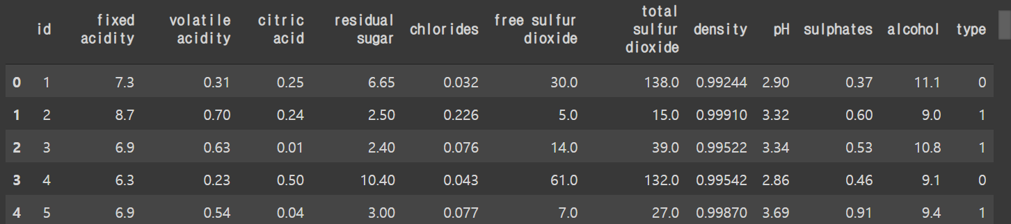
test.describe()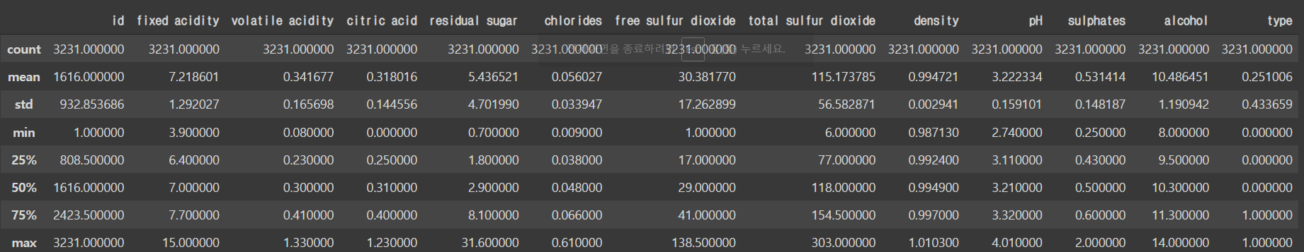
test.info()<class 'pandas.core.frame.DataFrame'>
RangeIndex: 3231 entries, 0 to 3230
Data columns (total 13 columns):
# Column Non-Null Count Dtype
--- ------ -------------- -----
0 id 3231 non-null int64
1 fixed acidity 3231 non-null float64
2 volatile acidity 3231 non-null float64
3 citric acid 3231 non-null float64
4 residual sugar 3231 non-null float64
5 chlorides 3231 non-null float64
6 free sulfur dioxide 3231 non-null float64
7 total sulfur dioxide 3231 non-null float64
8 density 3231 non-null float64
9 pH 3231 non-null float64
10 sulphates 3231 non-null float64
11 alcohol 3231 non-null float64
12 type 3231 non-null int64
dtypes: float64(11), int64(2)
memory usage: 328.3 KB# Define Test's X Variables
X_test = test.drop(['id'], axis=1)1.2.3 Submission
submission.head()
2 EDA
2.1 Correlation Matrix
corr = train.drop(columns=['id']).corr()

mask = np.triu(np.ones_like(corr, dtype=bool))

f, ax = plt.subplots(figsize=(12, 10))

cmap = sns.diverging_palette(230, 20, as_cmap=True)

sns.heatmap(corr, mask=mask, cmap=cmap, vmax=.3, center=0, annot=True,
            square=True, linewidths=.5, cbar_kws={"shrink": .5})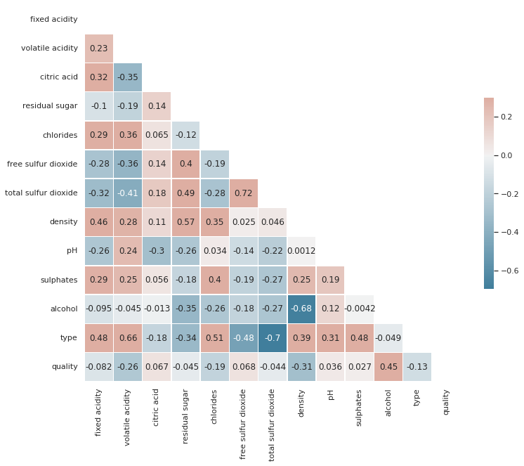
-
현재 quality의 등급과 상관 관계가 높은 값은 alcohol 밖에 없다.
-
두번째로 높은 alcohol의 경우 다른 feature들과의 상관관계가 상대적으로 높게 나온다.
2.2 Remove an Outlier
fig, axes = plt.subplots(1, 2, figsize=(2.33 * 10, 1 * 10))

for i, ax in enumerate(axes):
    if i == 0:
        sns.histplot(x= 'density', y= 'alcohol', bins=50, ax= ax, hue= 'quality',data= train)
        ax.add_patch(patches.Ellipse((1.0385, 11.7), .001, .5, color='r', fill=False))
    else:
        sns.histplot(x= 'density', y= 'alcohol', bins=50, ax= ax, hue= 'type',data= train)
        ax.add_patch(patches.Ellipse((1.0385, 11.7), .001, .5, color='r', fill=False))

axes[0].set_title('divided with quality', fontsize=20)
axes[1].set_title('divided with type', fontsize=20)
fig.suptitle('density & alcohol hist plot', fontsize= 40)
plt.show()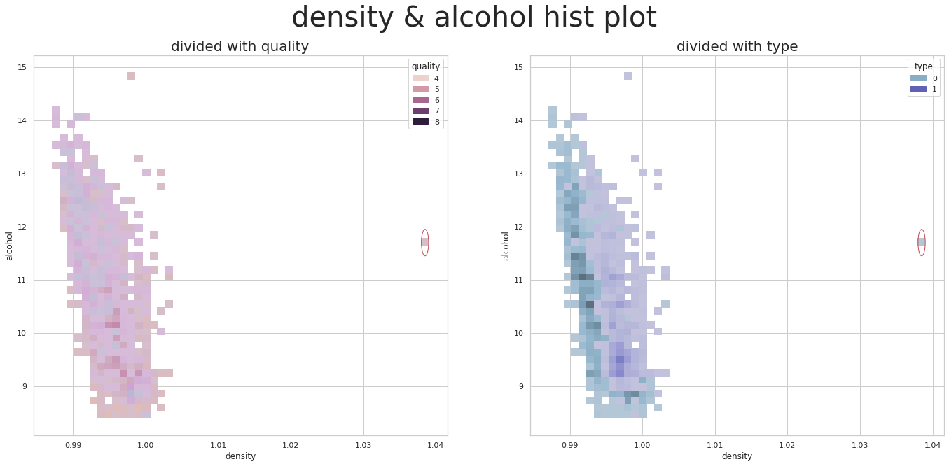
-
현재 Dacon에 재공된 기본 EDA에서 보여주는 그래프를 보면 이상치가 보여진다.
https://dacon.io/competitions/official/235840/codeshare/3779?page=1&dtype=recent
-
density 에서의 아웃라이어를 제거한 후 데이터 분석을 하는것이 좋을 것으로 보인다.
plt.boxplot(train['density'])
plt.show()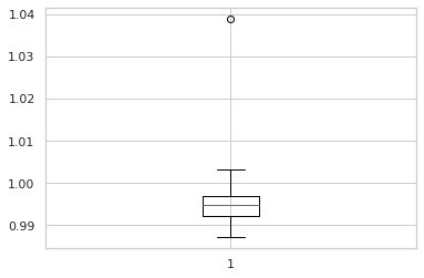
train[train['density'] > 1.03]
- train 에서 index 1368를 제거하여 준다.
train.drop([1368], inplace=True)plt.boxplot(train['density'])
plt.show()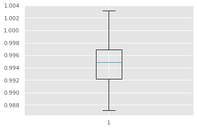
- Outlier 제거가 확인된다
2.3 Quality Distribution
counted_values = train['quality'].value_counts()
plt.style.use('ggplot')
plt.figure(figsize=(12, 10))
plt.title('class counting', fontsize = 30)
value_bar_ax = sns.barplot(x=counted_values.index, y=counted_values)
value_bar_ax.tick_params(labelsize=20)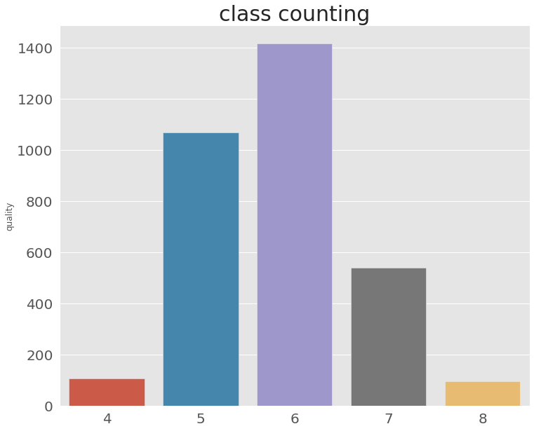
-
제공된 EDA에 의하면 현재 주어진 데이터의 와인 quality는 6에 치중되어 있고 4와 8에는 주어진 데이터 값이 적다.
https://dacon.io/competitions/official/235840/codeshare/3779?page=1&dtype=recent
-
실제로 proportional-odds 모델을 사용할 경우 4와 8의 예측 값이 떨어진다.
https://dacon.io/competitions/official/235840/codeshare/3780?page=1&dtype=recent
3 Classification Modeling
3.1 LGBM Classifier
# Google Colab을 사용시 optuna 설치가 필요하다.
!pip install optuna
# import library
## LGBM
from lightgbm import LGBMClassifier
## K-folds
from sklearn.model_selection import StratifiedKFold
## Optuna
from optuna.samplers import TPESampler
import optuna.integration.lightgbm as lgb# Splits to X and y
X = train.drop(['id', 'quality'], axis=1)
y = train.quality-4
## LGBM CV에 넣기 전에 quality의 값을 0~4 값으로 변환 시켜야
## LightGBMTunerCV 가 작동된다.
# Generate dtrain for LGBM-CV
dtrain = lgb.Dataset(X, label=y)params = {
"objective": "multiclass",
"num_class": 5,
"metric": "multi_logloss",
"verbosity": -1,
"boosting_type": "gbdt",
'learning_rate': 0.03,
'random_state': 314
}# LGBM K-CV 현재 10 Folds로 설정되어 있다.
tuner = lgb.LightGBMTunerCV(
params, dtrain, verbose_eval=100, early_stopping_rounds=100,
folds=StratifiedKFold(n_splits=10, shuffle=True))
tuner.run() 0%| | 0/7 [00:00<?, ?it/s]
feature_fraction, val_score: inf: 0%| | 0/7 [00:00<?, ?it/s][100] cv_agg's multi_logloss: 0.961617 + 0.0208537
[200] cv_agg's multi_logloss: 0.929495 + 0.0322221
[300] cv_agg's multi_logloss: 0.936998 + 0.0391396- 계산을 시작하면 위와 같은 코드가 뜨고 10 folds의 경우 40분정도 소비된다.
# Print the Best Score
tuner.best_score
0.8994136421217034
# Print the best_parameters
lgbm_params = tuner.best_params
tuner.best_params
{'bagging_fraction': 1.0,
'bagging_freq': 0,
'boosting_type': 'gbdt',
'feature_fraction': 0.5,
'feature_pre_filter': False,
'lambda_l1': 0.0,
'lambda_l2': 0.0,
'learning_rate': 0.03,
'metric': 'multi_logloss',
'min_child_samples': 20,
'num_class': 5,
'num_leaves': 245,
'objective': 'multiclass',
'random_state': 314,
'verbosity': -1}# LGBMClassifier 모델 학습
model_lgbm = LGBMClassifier(**lgbm_params)
studied_lgbm = model_lgbm.fit(X, y)# X_test 학습
submission['quality'] = studied_lgbm.predict(X_test)submission.quality = submission.quality+4
## 0~4로 변환된 값을 다시 4~8 값으로 변환한다.submission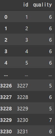
# Submission 저장하기
submission_path = ".../submission/"
submission.to_csv(submission_path+'lgbmSubmission.csv', sep=',', index=False)
Submission 확인
counted_values = submission['quality'].value_counts()
plt.style.use('ggplot')
plt.figure(figsize=(12, 10))
plt.title('class counting', fontsize = 30)
value_bar_ax = sns.barplot(x=counted_values.index, y=counted_values)
value_bar_ax.tick_params(labelsize=20)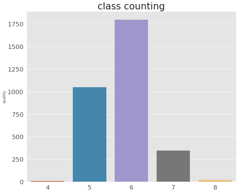
-
데이콘에 제공된 기본 코드와 비교하여 봤을때 LGBM Classifier를 사용시 quality 4와 8에 대한 예측값은 나왔다.
https://dacon.io/competitions/official/235840/codeshare/3780?page=1&dtype=recent
-
accuracy값 향상을 위해선 다른 모델을 사용하거나 regressor를 사용후 소숫점 자리를 처리하는 것이 좋을 것으로 보인다.