대회 설명

목적
- 제주시 내 택배 운송 데이터를 이용하여 운송량 예측 AI 개발
평가 산식 : RMSE
데이터 설명
- index : 인덱스
- SENDSPG_INNB : 송하인격자공간고유번호
- REC_SPG_INNB : 수하인 격자공간고유번호
- DLGD_LCLS_NM : 카테고리대
- DLGD_MCLS_NM : 카테고리중
- INVC_CONT : 운송장 건 수
1 Setting
1.1 Import Libraries
import pandas as pd
import numpy as np
import matplotlib.pyplot as plt
import seaborn as sns
from matplotlib import patches
# seaborn setting
sns.set_theme(style='whitegrid')
sns.set_palette("twilight")1.2 Import Datas
# define data path
data_path = ".../data/"

# Training and Testing Sets
train = pd.read_csv(data_path + "train_df.csv", encoding='cp949')
test = pd.read_csv(data_path + "test_df.csv", encoding='cp949')
# Submission
submission = pd.read_csv(data_path + "sample_submission.csv")
1.2.1 Training Set
train.head()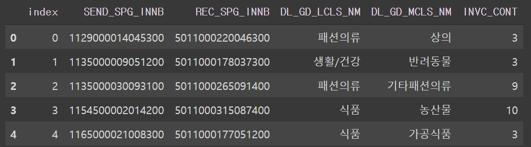
train.info()<class 'pandas.core.frame.DataFrame'>
RangeIndex: 32000 entries, 0 to 31999
Data columns (total 6 columns):
# Column Non-Null Count Dtype
--- ------ -------------- -----
0 index 32000 non-null int64
1 SEND_SPG_INNB 32000 non-null int64
2 REC_SPG_INNB 32000 non-null int64
3 DL_GD_LCLS_NM 32000 non-null object
4 DL_GD_MCLS_NM 32000 non-null object
5 INVC_CONT 32000 non-null int64
dtypes: int64(4), object(2)
memory usage: 1.5+ MB-
송하인과 수하인의 경우 16자리의 숫자중 앞의 4자리가 격자 번호이다.
-
따라서 앞의 4자리 수만을 가지고 categorical 형식으로 바꾸어 진행하는 것이 좋을 것으로 보인다.
# convert int to str
train['SEND_SPG_INNB'] = train['SEND_SPG_INNB'].apply(str)
train['REC_SPG_INNB'] = train['REC_SPG_INNB'].apply(str)

# slice the index numbers
train['SEND_SPG_INNB'] = train['SEND_SPG_INNB'].str.slice(start=0, stop=4)
train['REC_SPG_INNB'] = train['REC_SPG_INNB'].str.slice(start=0, stop=4)
train.describe(include='all')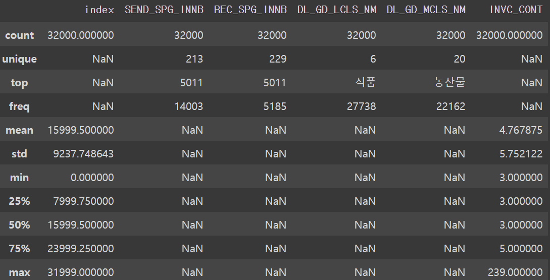
1.2.2 Testing Set
# convert int to str
test['SEND_SPG_INNB'] = test['SEND_SPG_INNB'].apply(str)
test['REC_SPG_INNB'] = test['REC_SPG_INNB'].apply(str)

# slice the index numbers
test['SEND_SPG_INNB'] = test['SEND_SPG_INNB'].str.slice(start=0, stop=4)
test['REC_SPG_INNB'] = test['REC_SPG_INNB'].str.slice(start=0, stop=4)
test.head()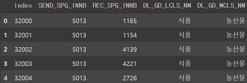
test.info()<class 'pandas.core.frame.DataFrame'>
RangeIndex: 4640 entries, 0 to 4639
Data columns (total 5 columns):
# Column Non-Null Count Dtype
--- ------ -------------- -----
0 index 4640 non-null int64
1 SEND_SPG_INNB 4640 non-null object
2 REC_SPG_INNB 4640 non-null object
3 DL_GD_LCLS_NM 4640 non-null object
4 DL_GD_MCLS_NM 4640 non-null object
dtypes: int64(1), object(4)
memory usage: 181.4+ KBtest.describe(include='all')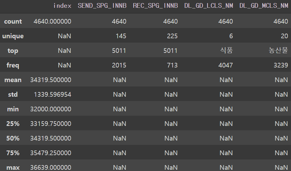
1.2.3 Submission
submission.head()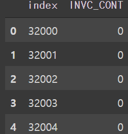
2 EDA
2.1 SEND_SPG_INNB(송하인)
plt.subplot(2, 1, 1)
order_send = train.groupby('SEND_SPG_INNB').count()['INVC_CONT'].sort_values()
order_send_plot = order_send.tail(10).plot(kind='bar', figsize=(30, 10))
order_send_plot.set_xlabel('Top 10 SEND_SPG_INNB', fontsize=13)
order_send_plot.set_ylabel('Number of Orders', fontsize=13)

plt.subplot(2, 1, 2)
order_send_total = train.groupby('SEND_SPG_INNB').sum()['INVC_CONT'].sort_values()
order_send_total_plot = order_send_total.tail(10).plot(kind='bar', figsize=(30, 10))
order_send_total_plot.set_xlabel('Top 10 SEND_SPG_INNB', fontsize=13)
order_send_total_plot.set_ylabel('Total Number of Ordered Items', fontsize=13)

plt.show()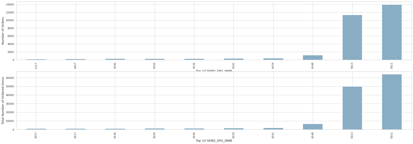
print(order_send.tail(10))
print(order_send_total.tail(10))
SEND_SPG_INNB
1117 175
4157 209
4146 267
4150 270
4136 272
4141 363
4159 395
4148 1203
5013 11341
5011 14003
Name: INVC_CONT, dtype: int64
SEND_SPG_INNB
4157 1214
4117 1299
4136 1317
4150 1481
4146 1610
4159 1841
4141 1896
4148 6588
5013 49848
5011 64098
Name: INVC_CONT, dtype: int64- 상위 두개의 송하인을 제외하면 주문 건수가 높다고 주문량이 높게 나오지는 않는다.
2.2 REC_SPG_INNB(수하인)
plt.subplot(2, 1, 1)
order_recv = train.groupby('REC_SPG_INNB').count()['INVC_CONT'].sort_values()
order_recv_plot = order_recv.tail(10).plot(kind='bar', figsize=(30, 10))
order_recv_plot.set_xlabel('Top 10 REC_SPG_INNB', fontsize=13)
order_recv_plot.set_ylabel('Number of Recived Items', fontsize=13)

plt.subplot(2, 1, 2)
order_recv_total = train.groupby('REC_SPG_INNB').sum()['INVC_CONT'].sort_values()
order_recv_total_plot = order_recv_total.tail(10).plot(kind='bar', figsize=(30, 10))
order_recv_total_plot.set_xlabel('Top 10 REC_SPG_INNB', fontsize=13)
order_recv_total_plot.set_ylabel('Total Number of Recived Items', fontsize=13)

plt.show()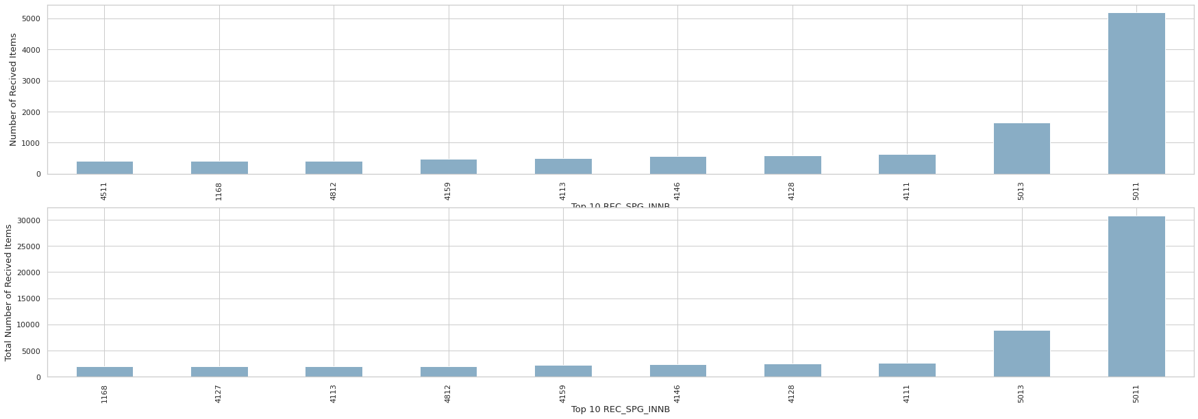
print(order_recv.tail(10))
print(order_recv_total.tail(10))
REC_SPG_INNB
4511 413
1168 416
4812 422
4159 487
4113 493
4146 564
4128 587
4111 631
5013 1648
5011 5185
Name: INVC_CONT, dtype: int64
REC_SPG_INNB
1168 1937
4127 1939
4113 1959
4812 1990
4159 2303
4146 2351
4128 2489
4111 2667
5013 8883
5011 30796
Name: INVC_CONT, dtype: int64- 수하인의 경우 상위 4개의 수하인을 제외하면 주문 횟수가 높다고 전체 주문량이 높게 나오진 않는다.
2.3 DL_GD_LCLS_NM(카테고리 대)
catb_count = train.groupby('DL_GD_LCLS_NM').count()['INVC_CONT'].sort_values(ascending=False)
catb_count_total = train.groupby('DL_GD_LCLS_NM').sum()['INVC_CONT'].sort_values(ascending=False)

print(catb_count)
print(catb_count_total)
DL_GD_LCLS_NM
식품 27738
생활/건강 2020
여행/문화 1192
패션의류 582
디지털/가전 241
화장품/미용 227
Name: INVC_CONT, dtype: int64
DL_GD_LCLS_NM
식품 129209
생활/건강 10924
여행/문화 5911
패션의류 3887
디지털/가전 1578
화장품/미용 1063
Name: INVC_CONT, dtype: int64- 카테고리의 경우 주문 건수가 높을경우 전체 주문량 또한 높게 나온다.
2.4 DL_GD_MCLS_NM(카테고리 중)
catm_count = train.groupby('DL_GD_MCLS_NM').count()['INVC_CONT'].sort_values(ascending=False)
catm_count_total = train.groupby('DL_GD_MCLS_NM').sum()['INVC_CONT'].sort_values(ascending=False)

catm_count.rename('catm_count', inplace=True)
catm_count_total.rename('catm_count_total', inplace=True)

cat_count = pd.concat([catm_count, catm_count_total], axis=1)
cat_count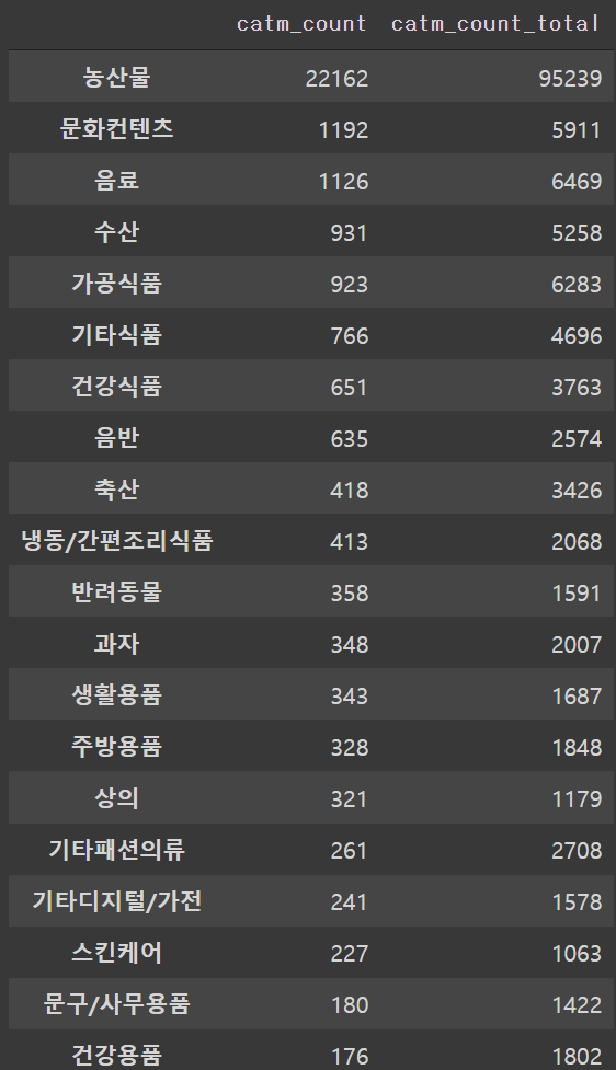
- 카테고리 중의 경우에도 주문 건수가 높을 수록 총 주문량이 높게 나온다.
3 Feature Engineering
- 현재 데이터의 특성을 보면 송하인과 수하인의 경우 주문 건수가 높다고 전체 주문량이 높게 나오지는 않았다.
- 반면에 카테고리의 경우 주문 건수가 높을 경우 전체 주문량 또한 높았다.
3.1 SEND_SPG_INNB 평균 값
avg_send = order_send_total/order_send
avg_send.rename('avg_send', inplace=True)
avg_send = avg_send.reset_index().rename(columns={'index': 'SEND_SPG_INNB'})
# merge to train & test
train = pd.merge(left=train, right=avg_send,
how='left', on=['SEND_SPG_INNB'])
test = pd.merge(left=test, right=avg_send,
how='left', on=['SEND_SPG_INNB'])
train.info()<class 'pandas.core.frame.DataFrame'>
Int64Index: 32000 entries, 0 to 31999
Data columns (total 8 columns):
# Column Non-Null Count Dtype
--- ------ -------------- -----
0 index 32000 non-null int64
1 SEND_SPG_INNB 32000 non-null object
2 REC_SPG_INNB 32000 non-null object
3 DL_GD_LCLS_NM 32000 non-null object
4 DL_GD_MCLS_NM 32000 non-null object
5 INVC_CONT 32000 non-null int64
6 avg_send_x 32000 non-null float64
7 avg_send_y 32000 non-null float64
dtypes: float64(2), int64(2), object(4)
memory usage: 2.2+ MBtest.info()<class 'pandas.core.frame.DataFrame'>
Int64Index: 4640 entries, 0 to 4639
Data columns (total 7 columns):
# Column Non-Null Count Dtype
--- ------ -------------- -----
0 index 4640 non-null int64
1 SEND_SPG_INNB 4640 non-null object
2 REC_SPG_INNB 4640 non-null object
3 DL_GD_LCLS_NM 4640 non-null object
4 DL_GD_MCLS_NM 4640 non-null object
5 avg_send_x 4637 non-null float64
6 avg_send_y 4637 non-null float64
dtypes: float64(2), int64(1), object(4)
memory usage: 290.0+ KB3.2 REC_SPG_INNB 평균 값
avg_rec = order_recv_total/order_recv
avg_rec.rename('avg_rec', inplace=True)
avg_rec = avg_rec.reset_index().rename(columns={'index': 'REC_SPG_INNB'})
# merge to train & test
train = pd.merge(left=train, right=avg_rec,
how='left', on=['REC_SPG_INNB'])
test = pd.merge(left=test, right=avg_rec,
how='left', on=['REC_SPG_INNB'])3.3 카테고리 대 평균 값
avg_catb = catb_count_total/catb_count
avg_catb.rename('avg_catb', inplace=True)
avg_catb = avg_catb.reset_index().rename(columns={'index': 'DL_GD_LCLS_NM'})
# merge to train & test
train = pd.merge(left=train, right=avg_catb,
how='left', on=['DL_GD_LCLS_NM'])
test = pd.merge(left=test, right=avg_catb,
how='left', on=['DL_GD_LCLS_NM'])3.4 카테고리 중 평균 값
avg_catm = catm_count_total/catm_count
avg_catm.rename('avg_catm', inplace=True)
avg_catm = avg_catm.reset_index().rename(columns={'index': 'DL_GD_MCLS_NM'})

# merge to train and test
train = pd.merge(left=train, right=avg_catm,
                 how='left', on=['DL_GD_MCLS_NM'])

test = pd.merge(left=test, right=avg_catm,
                 how='left', on=['DL_GD_MCLS_NM'])
4 After Feature Engineering
4.1 Correlation Matrix
# Compute the correlation matrix
corr = train.drop(['index'], axis=1).corr()

# Generate a mask for the upper triangle
mask = np.triu(np.ones_like(corr, dtype=bool))

# Set up the matplotlib figure
f, ax = plt.subplots(figsize=(11, 9))

# Generate a custom diverging colormap
cmap = sns.diverging_palette(230, 20, as_cmap=True)

# Draw the heatmap with the mask and correct aspect ratio
sns.heatmap(corr, mask=mask, cmap=cmap, vmax=.3, center=0, annot=True,
            square=True, linewidths=.5, cbar_kws={"shrink": .5})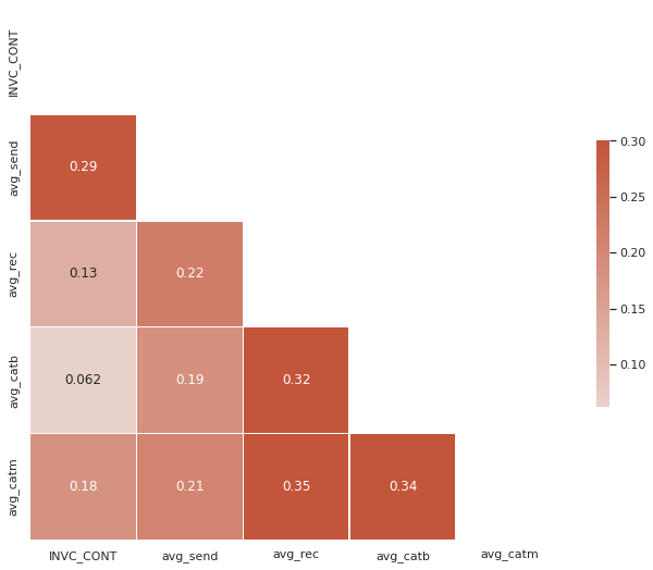
4.2 Spliting the data sets to X and y
# Training X and y
X = train.drop(['INVC_CONT', 'index', 'SEND_SPG_INNB', 'REC_SPG_INNB',
                'DL_GD_LCLS_NM', 'DL_GD_MCLS_NM'], axis=1)
y = train.INVC_CONT

# Testing X
X_test = test.drop(['index', 'SEND_SPG_INNB', 'REC_SPG_INNB',
                    'DL_GD_LCLS_NM', 'DL_GD_MCLS_NM'], axis=1)