0. SQL로 데이터 합치기

• 데이터는 총 5개의 csv 파일로 나누어져 있다.
• 우선 각 파일을 아래의 SQL조건으로 합쳤다.

    select
        d1.*,
        d2.aisle_id, d2.department_id,
        d3.department,
        d4.aisle,
        d5.order_number, d5.order_dow, d5.order_hour_of_day,
        d5.days_since_prior_order, d5.eval_set
    from 
        test.order_products as d1
        inner join test.products as d2
            on d1.product_id = d2.product_id
        inner join test.departments as d3
            on d2.department_id = d3.department_id 
        inner join test.aisles as d4
            on d2.aisle_id = d4.aisle_id
        inner join test.orders as d5
            on d5.order_id = d1.order_id;

• 데이터에서 재품 이름을 가뎌오지 않았다.
• 총 13개의 variable이 만들어졌다.
• inner join 을 했을시 데이터 길이가 1,048,576에서 422,287이 되었다.

1. 데이터 분석의 목적과 방향성

• 데이터 분석의 목표

  Instacart 온라인 마켓에 식료품 아이탬에 따른 재주문 여부를 예측하는 것이다.

• 변수값 설명

  현재 데이터엔 13개의 variable 이 있다.

  Y variable은 'reordered' 이고 bionary scale 이다.

  나머지 12개의 variable은 X variable로 둔다.

  add_to_cart_order 는 정확한 정보는 없지만 cart에 들어있는 아이템 계수로 보인다.

  order_id는 주문 index다.

  product_id는 제품 종류에 따른 번호이다 각 품목에 대한 이름을 id로 표시해 놓았다.

  aisle_id 는 제품이 display되어있는 색션으로 134개의 level이 있다.

  aisle는 색션의 이름 정보이다.

  department_id 는 식료품의 종류로 21개의 level이 있다.

  department는 식료품 종류에 대한 str정보이다.(마찬가지로 21개의 level이 있다.

  order_hour_of_day 는 주문 시간 정보이다.

  days_since_prior_order 는 재주문을 하는데 걸린 시간이다. 0~30이 있다.

  order_dow 는 주문 요일로 0~6의 인덱스로 되어있고 어느 요일이 어떻게 인덱싱 되었는지는 모른다.

2. EDA Setting

2.1 Library 불러오기

import pandas as pd
import numpy as np
import matplotlib.pyplot as plt
import seaborn as sns

sns.set_theme(style='whitegrid')
sns.set_palette("twilight")

2.2 데이터 불러오기

from google.colab import files
myfile = files.upload()

import io

train = pd.read_csv('mydata.csv')

type(train)

pandas.core.frame.DataFrame

train.head()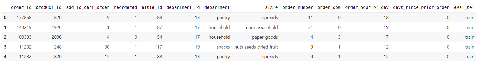

train.info()
## No NULL value in the data

<class 'pandas.core.frame.DataFrame'>
RangeIndex: 422286 entries, 0 to 422285
Data columns (total 13 columns):
 #   Column                  Non-Null Count   Dtype 
---  ------                  --------------   ----- 
 0   order_id                422286 non-null  int64 
 1   product_id              422286 non-null  int64 
 2   add_to_cart_order       422286 non-null  int64 
 3   reordered               422286 non-null  int64 
 4   aisle_id                422286 non-null  int64 
 5   department_id           422286 non-null  int64 
 6   department              422286 non-null  object
 7   aisle                   422286 non-null  object
 8   order_number            422286 non-null  int64 
 9   order_dow               422286 non-null  int64 
 10  order_hour_of_day       422286 non-null  int64 
 11  days_since_prior_order  422286 non-null  int64 
 12  eval_set                422286 non-null  object
dtypes: int64(10), object(3)
memory usage: 41.9+ MB
train.describe(include='all')

3. EDA

3.1 Department id의 재주문

• 현재 Instacart에서 원하는 정보는 Product에 따른 재구메 정보이다.
• Department는 Product를 그룹별로 묶어놓은 것이다.
• Department id는 21개의 level로 되어있다.

# barplot of reordered by department_id 
plt.figure(figsize=(12,12))
dep_bar = sns.barplot(x='department_id',
                      y='reordered',
                      data=train)
# xlab and ylab
dep_bar.set_xlabel('Department ID', fontsize=13)
dep_bar.set_ylabel('Percentage of Reordered', fontsize=13)
dep_bar.set_title('Barplot of Reordered by Department ID', fontsize=16)
plt.show()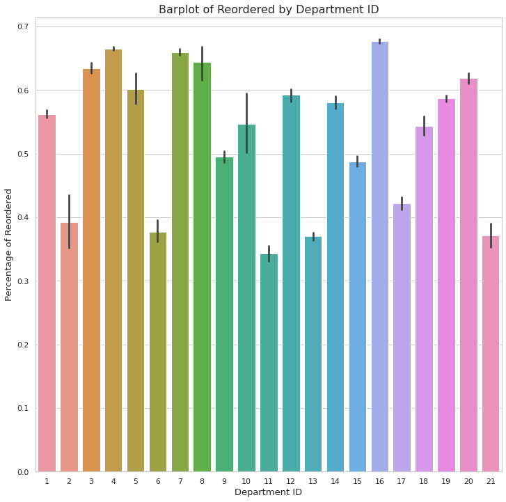

• 13개의 product에 대해 재주문율이 50% 이상이다.
• 위의 product_id 가 1, 3, 4, 5, 7, 8, 10, 12, 14, 16, 18, 19, 20 이 재구매율이 50% 이상이다.

1	3	4	5	7	8	10	12	14	16	18	19	20
Frozen	Bakery	Produce	Alcohol	Beverages	Pets	Bulk	Meat and Seafood	Breakfast	Dairy eggs	Babies	Snacks	Deli

# histplot of total number of order by department_id 
plt.figure(figsize=(12,12))
dep_bar = sns.histplot(x='department_id',
                       bins=21,
                      data=train)
# xlab and ylab
dep_bar.set_xlabel('Department ID', fontsize=13)
dep_bar.set_ylabel('Total Number of Order', fontsize=13)
dep_bar.set_title('Histplot of Ordered by Department ID', fontsize=16)
plt.show()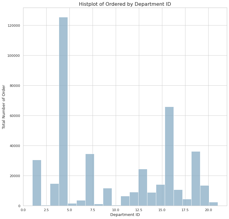

• 현재 전체에서 재주물율이 높은 품목은 21개 중에 13개 이다.
• 그러나 전체 판매합계를 보면 5개 품목(4, 16, 19, 7, 1 높은 순으로)의 주문량이 높다.
• 따라서 후에 4, 16, 19, 7, 1에 따른 EDA를 진행하는 것이 효율적으로 보인다.

4	16	19	7	1
Produce	Dairy eggs	Snacks	Beverages	Frozen

3.2 Product 에 따른 재주문

• 현재 Instacart 에서 원하는건 Product에 따른 재주문에 대한 정보를 얻는 것이다.
• 우선 전체 product의 주문과 재주문을 보자.

# product_id에 대해 오름차순으로 정렬
prod_sort = train['product_id']
prod_sort = prod_sort.sort_values()

prod_sort

315587        1
116308        1
200210        1
97413         1
344722        1
          ...  
219761    49683
350740    49683
83012     49686
316142    49688
181193    49688
Name: product_id, Length: 422286, dtype: int64

# index 다시부여하기
prod_sort = prod_sort.reset_index()
prod_sort

	index	product_id
0	315587	1
1	116308	1
2	200210	1
3	97413	1
4	344722	1
...	...	...
422281	219761	49683
422282	350740	49683
422283	83012	49686
422284	316142	49688
422285	181193	49688
422286 rows × 2 columns

# drop the index column
prod_sort.drop('index', axis=1, inplace=True)
prod_sort.head()

product_id
0	1
1	1
2	1
3	1
4	1

prod_sort.plot()
plt.show()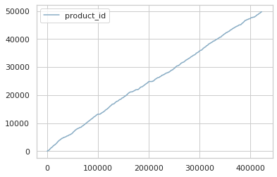

• 현재 plot이 보여주는 값은 product의 종류에 따라 linear형식으로 판매량이 높은것으로 보인다.

3.2.1 Department에 따른 Product 주문

• 현재 Product는 49,688개가 존재한다.
• 이때 상위 재품들만을 보기 보단 상위 5개의 Department에 따른 Product의 판매량과 재판매량을 보는것이 효율적일 것으로 판단된다.

# product_id convert int to object
train['product_id'] = train['product_id'].astype('object')
train.info()

<class 'pandas.core.frame.DataFrame'>
RangeIndex: 422286 entries, 0 to 422285
Data columns (total 13 columns):
 #   Column                  Non-Null Count   Dtype 
---  ------                  --------------   ----- 
 0   order_id                422286 non-null  int64 
 1   product_id              422286 non-null  object
 2   add_to_cart_order       422286 non-null  int64 
 3   reordered               422286 non-null  int64 
 4   aisle_id                422286 non-null  int64 
 5   department_id           422286 non-null  int64 
 6   department              422286 non-null  object
 7   aisle                   422286 non-null  object
 8   order_number            422286 non-null  int64 
 9   order_dow               422286 non-null  int64 
 10  order_hour_of_day       422286 non-null  int64 
 11  days_since_prior_order  422286 non-null  int64 
 12  eval_set                422286 non-null  object
dtypes: int64(9), object(4)
memory usage: 41.9+ MB

# 상위 다섯개 Department의 전체주문에 대한 데이터 지정
dep4 = train[train['department_id']==4]
dep16 = train[train['department_id']==16]
dep19 = train[train['department_id']==19]
dep7 = train[train['department_id']==7]
dep1 = train[train['department_id']==1]

# Department에 따른 product 정렬
dep4_prod = dep4.groupby('product_id').count()['reordered'].sort_values()
dep16_prod = dep16.groupby('product_id').count()['reordered'].sort_values()
dep19_prod = dep19.groupby('product_id').count()['reordered'].sort_values()
dep7_prod = dep7.groupby('product_id').count()['reordered'].sort_values()
dep1_prod = dep1.groupby('product_id').count()['reordered'].sort_values()

# Department에 따른 product 재주문 정렬
dep4_prod_re = dep4.groupby('product_id').sum()['reordered'].sort_values()
dep16_prod_re = dep16.groupby('product_id').sum()['reordered'].sort_values()
dep19_prod_re = dep19.groupby('product_id').sum()['reordered'].sort_values()
dep7_prod_re = dep7.groupby('product_id').sum()['reordered'].sort_values()
dep1_prod_re = dep1.groupby('product_id').sum()['reordered'].sort_values()

# department_id 4의 product_id의 상위 10개에 대한 barplot
plt.subplot(1, 2, 1)
dep4_prod_plot = dep4_prod.tail(10).plot(kind='bar', figsize=(12, 12))
dep4_prod_plot.set_xlabel("Department 4's Top 10 Products", fontsize=13)
dep4_prod_plot.set_ylabel("Total Number of Orders", fontsize=13)
dep4_prod_plot.set_title("Number of Orders by Products", fontsize=15)
dep4_prod_plot.set_xticklabels(labels=dep4_prod.index, rotation=45)
# reordered 에 대한 Top 10
plt.subplot(1, 2, 2)
dep4_prod_re_plot = dep4_prod_re.tail(10).plot(kind='bar', figsize=(12, 12))
dep4_prod_re_plot.set_xlabel("Department 4's Top 10 Reordered Products", fontsize=13)
dep4_prod_re_plot.set_ylabel("Total Number of Orders", fontsize=13)
dep4_prod_re_plot.set_title("Number of Reorders by Products", fontsize=15)
dep4_prod_re_plot.set_xticklabels(labels=dep4_prod.index, rotation=45)
plt.show()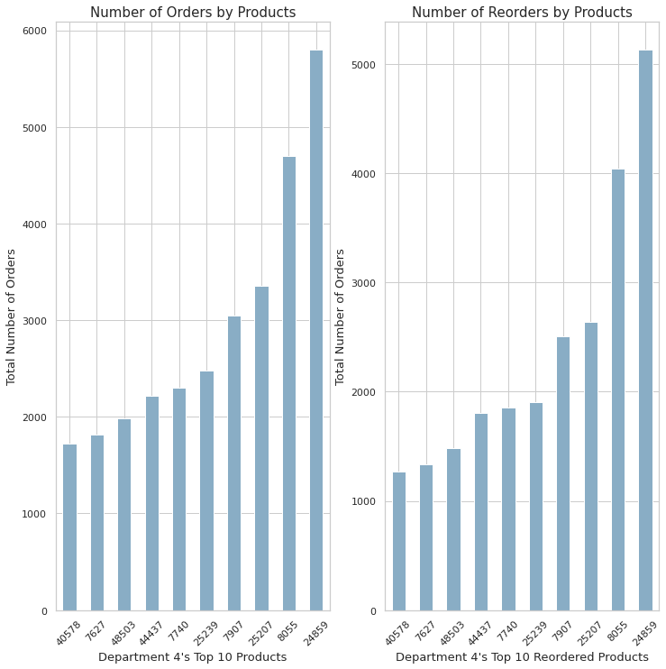

• 위의 10개의 재품에 대해 전체 주문량과 재주문량 순위가 매겨졌다.
• Department 4의 Top 10 주문과 재주문은 같은 순위를 가지고 있다.

# department_id 16의 product_id의 상위 10개에 대한 barplot
plt.subplot(1, 2, 1)
dep16_prod_plot = dep16_prod.tail(10).plot(kind='bar', figsize=(12, 12))
dep16_prod_plot.set_xlabel("Department 16's Top 10 Products", fontsize=13)
dep16_prod_plot.set_ylabel("Total Number of Orders", fontsize=13)
dep16_prod_plot.set_title("Number of Orders by Products", fontsize=15)
dep16_prod_plot.set_xticklabels(labels=dep16_prod.index, rotation=45)
# reordered 에 대한 Top 10
plt.subplot(1, 2, 2)
dep16_prod_re_plot = dep16_prod_re.tail(10).plot(kind='bar', figsize=(12, 12))
dep16_prod_re_plot.set_xlabel("Department 16's Top 10 Reordered Products", fontsize=13)
dep16_prod_re_plot.set_ylabel("Total Number of Reorders", fontsize=13)
dep16_prod_re_plot.set_title("Number of Reorders by Products", fontsize=15)
dep16_prod_re_plot.set_xticklabels(labels=dep16_prod.index, rotation=45)
plt.show()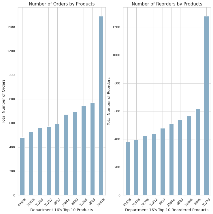

• 위의 10개의 재품에 대해 전체 주문량과 재주문량 순위가 매겨졌다.
• Department 16의 Top 10 주문과 재주문은 같은 순위를 가지고 있다.

# department_id 19의 product_id의 상위 10개에 대한 barplot
plt.subplot(1, 2, 1)
dep19_prod_plot = dep19_prod.tail(10).plot(kind='bar', figsize=(12, 12))
dep19_prod_plot.set_xlabel("Department 19's Top 10 Products", fontsize=13)
dep19_prod_plot.set_ylabel("Total Number of Orders", fontsize=13)
dep19_prod_plot.set_title("Number of Orders by Products", fontsize=15)
dep19_prod_plot.set_xticklabels(labels=dep19_prod.index, rotation=45)
# reordered 에 대한 Top 10
plt.subplot(1, 2, 2)
dep19_prod_re_plot = dep19_prod_re.tail(10).plot(kind='bar', figsize=(12, 12))
dep19_prod_re_plot.set_xlabel("Department 19's Top 10 Reordered Products", fontsize=13)
dep19_prod_re_plot.set_ylabel("Total Number of Reorders", fontsize=13)
dep19_prod_re_plot.set_title("Number of Reorders by Products", fontsize=15)
dep19_prod_re_plot.set_xticklabels(labels=dep19_prod.index, rotation=45)
plt.show()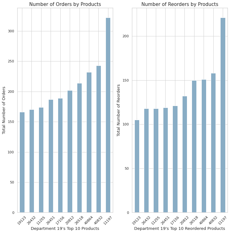

• 위의 10개의 재품에 대해 전체 주문량과 재주문량 순위가 매겨졌다.
• Department 19의 Top 10 주문과 재주문은 같은 순위를 가지고 있다.

# department_id 7의 product_id의 상위 10개에 대한 barplot
plt.subplot(1, 2, 1)
dep7_prod_plot = dep7_prod.tail(10).plot(kind='bar', figsize=(12, 12))
dep7_prod_plot.set_xlabel("Department 7's Top 10 Products", fontsize=13)
dep7_prod_plot.set_ylabel("Total Number of Orders", fontsize=13)
dep7_prod_plot.set_title("Number of Orders by Products", fontsize=15)
dep7_prod_plot.set_xticklabels(labels=dep7_prod.index, rotation=45)
# reordered 에 대한 Top 10
plt.subplot(1, 2, 2)
dep7_prod_re_plot = dep7_prod_re.tail(10).plot(kind='bar', figsize=(12, 12))
dep7_prod_re_plot.set_xlabel("Department 7's Top 10 Reordered Products", fontsize=13)
dep7_prod_re_plot.set_ylabel("Total Number of Reorders", fontsize=13)
dep7_prod_re_plot.set_title("Number of Reorders by Products", fontsize=15)
dep7_prod_re_plot.set_xticklabels(labels=dep7_prod.index, rotation=45)
plt.show()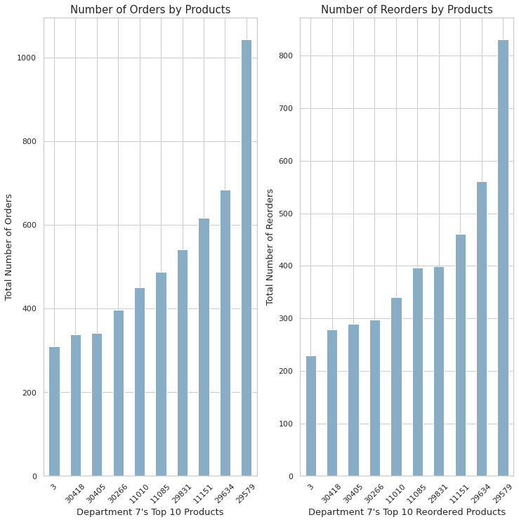

• 위의 10개의 재품에 대해 전체 주문량과 재주문량 순위가 매겨졌다.
• Department 7의 Top 10 주문과 재주문은 같은 순위를 가지고 있다.

# department_id 1의 product_id의 상위 10개에 대한 barplot
plt.subplot(1, 2, 1)
dep1_prod_plot = dep1_prod.tail(10).plot(kind='bar', figsize=(12, 12))
dep1_prod_plot.set_xlabel("Department 1's Top 10 Products", fontsize=13)
dep1_prod_plot.set_ylabel("Total Number of Orders", fontsize=13)
dep1_prod_plot.set_title("Number of Orders by Products", fontsize=15)
dep1_prod_plot.set_xticklabels(labels=dep1_prod.index, rotation=45)
# reordered 에 대한 Top 10
plt.subplot(1, 2, 2)
dep1_prod_re_plot = dep1_prod_re.tail(10).plot(kind='bar', figsize=(12, 12))
dep1_prod_re_plot.set_xlabel("Department 1's Top 10 Reordered Products", fontsize=13)
dep1_prod_re_plot.set_ylabel("Total Number of Reorders", fontsize=13)
dep1_prod_re_plot.set_title("Number of Reorders by Products", fontsize=15)
dep1_prod_re_plot.set_xticklabels(labels=dep1_prod.index, rotation=45)
plt.show()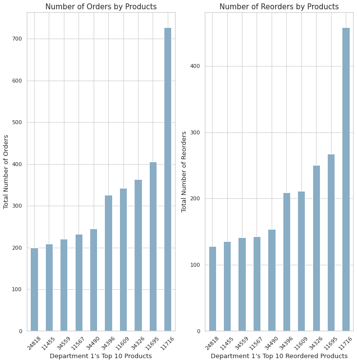

• 위의 10개의 재품에 대해 전체 주문량과 재주문량 순위가 매겨졌다.
• Department 1의 Top 10 주문과 재주문은 같은 순위를 가지고 있다.

3.2.2 Department와 Product에 대한 Insight

• 전체 주문과 재주문량이 Department 4 에서 가장 높게 나타났다.
• 절대적인 주문량이 높으면 재주문량 또한 높다.
• 상위 5개의 Department에 따른 재품들을 고객들에게 추천해주는 것이 효일적일 것으로 보인다.

3.3 days_since_prior_order 에 따른 재 구매율

• Instacart에는 monthly and annual 자동 주문기능이 있다.
• 웹사이트 상에 나와있는 홍보전략과 description을 보면 30일 단위로 재주문을 했을시 해택이 제공되는 것으로 보인다.

3.3.1 우선 일별로 재주문한 퍼센트에 대해 Barplot으로 살펴보다

# barplot of reordered by days_since_prior_order
plt.figure(figsize=(12,12))
dep_bar = sns.barplot(x='days_since_prior_order',
                      y='reordered',
                      data=train)
# xlab and ylab
dep_bar.set_xlabel('Reordered Days in 30', fontsize=13)
dep_bar.set_ylabel('Percentage of Reordered', fontsize=13)
dep_bar.set_title('Barplot of Reordered by Reordered Days in 30', fontsize=16)
plt.show()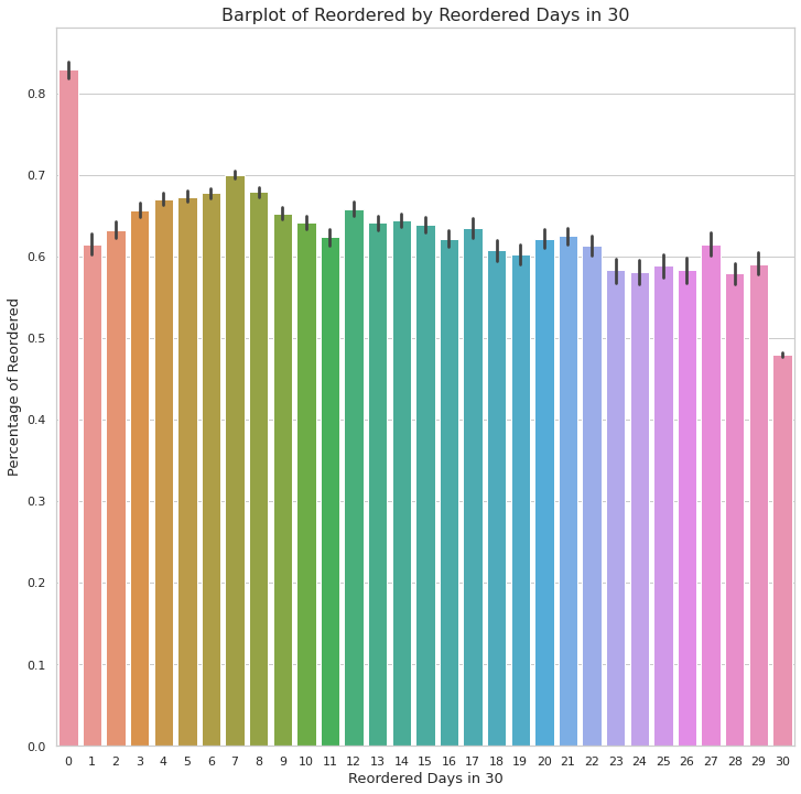

• 현재 비율로는 0일에 즉 제품을 주문한 날자에 재주문 하는 경우가 퍼센트 상으로 가장 높고 monthly order하는것이 가장 낮다.
• 이제 퍼센트가 아닌 카운트 상으로 어떻게 어떤 날자에 재주문량이 많은지 카운트 해보자

3.3.2 일별로 재주문한 건수에 대해 table 살펴보다

pd.crosstab(train['days_since_prior_order'], train['reordered'])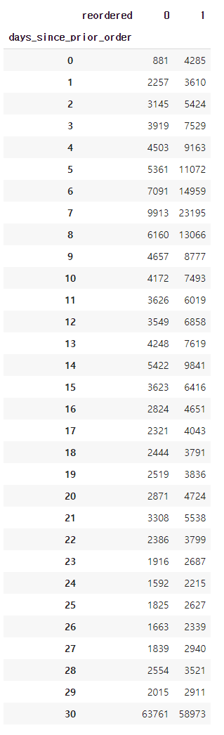

• 0일 즉 주문 당일 재주문은 퍼센트는 높지만 전체 카운트로 봤을때 높지가 않다.
• 반면에 30일 즉 monthly reorder는 퍼센트로는 낮지만 카운트로 봤을때 가장 높다.
• 따라서 monthly reorder가 Instacart에서 reorder 하는데 있어 가장 의미있는 수치를 보여준다.
• 다른 값들중 눈에 띄는 수치는 5~8일 이다.
• 5~8일 사이에 재주문 수치가 높은건 일주일 단위로 필요한 품목이 있는것으로 추측된다.

# 재주문에 대한 데이터 지정
reordered = train[train['reordered']==1]

# histplot of total number of reordered by days_since_prior_order
plt.figure(figsize=(12,12))
dep_hist = sns.histplot(x='days_since_prior_order',
                        bins=30,
                        data=reordered)
# xlab and ylab
dep_hist.set_xlabel('Reordered Days in 30', fontsize=13)
dep_hist.set_ylabel('Total Number of Reordered', fontsize=13)
dep_hist.set_title('Barplot of Reordered by Reordered Days in 30', fontsize=16)
plt.show()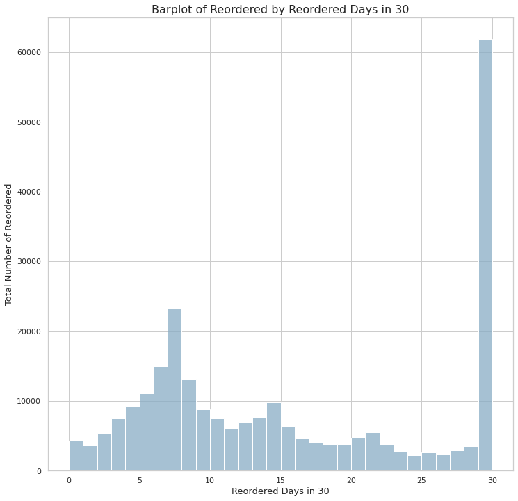

• 절대적으로 재주문량이 많은 날은 30일 이다.
• 그 다음 재주문량이 많은 날은 7일 이다.

3.3.3 재주문 날짜와 품목간의 상관관계

• 위의 결과들을 봤을때 일주일(5~8일) 단위로 주문 하는 품목과 한달 단위로 주문하는 품목이 있을것으로 보인다.
• 우선 일주일과 한달 단위와 전체 품목간의 관계를 보고 3.1에서 보여준 13개 품목이 재주문율이 높았는지 찾아보자.

# 일주일 과 한달에 대한 DataFrame 생성
fiveDays = train[(train['days_since_prior_order'] == 5) |
                 (train['days_since_prior_order'] == 6) |
                 (train['days_since_prior_order'] == 7) |
                 (train['days_since_prior_order'] == 8) |
                 (train['days_since_prior_order'] == 30)]

# 5일에 대한 department 카운트
pd.crosstab([fiveDays['department_id'],fiveDays['reordered'] ], fiveDays['days_since_prior_order'], margins=True, margins_name="Total")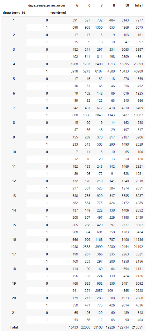

• 위에 카운트로 봤을시 조금 복잡하게 보인다.
• 위의 테이블을 퍼센트로 바꿔서 보자.

# 5일에 대한 department 퍼센트
table = pd.crosstab([fiveDays['department_id'],fiveDays['days_since_prior_order']], [fiveDays['reordered']], 
                    normalize='index')

pd.set_option('display.max_rows', None)
table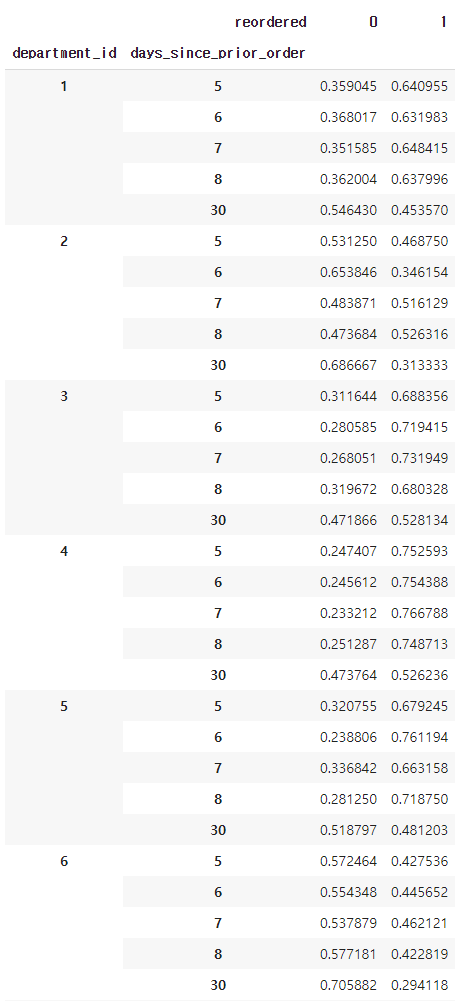

# 대표적으로 재구매가 많았던 날짜가 7일과 30일 임으로 두 날짜에 따른 재주문 율을 시각화 해보자
## 일주일
weekelyDays = train[(train['days_since_prior_order'] == 7) ]
weekelyTable = pd.crosstab([weekelyDays['department_id'],weekelyDays['days_since_prior_order']], [weekelyDays['reordered']], 
                    normalize='index')
## 30일
monthlyDays = train[(train['days_since_prior_order'] == 30) ]
monthlyTable = pd.crosstab([monthlyDays['department_id'],monthlyDays['days_since_prior_order']], [monthlyDays['reordered']], 
                    normalize='index')

plt.figure(figsize=(20,10)) ## plot에 대한  matplotlib 생성
plt.subplot(1,2,1)
sns.heatmap(weekelyTable, vmin=0.2, vmax=0.8, 
            linewidths=1, cmap="BuPu", cbar=False)

plt.subplot(1,2,2)
sns.heatmap(monthlyTable, vmin=0.2, vmax=0.8, 
            linewidths=1, cmap="BuPu")
plt.show()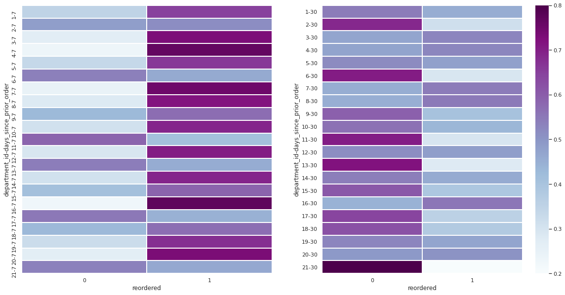

• 위의 좌측 테이블은 7일째에 재구매율에 대해 우측 테이블은 30일 째에 재구매율에 대해 보여준다.
• 짙은 보라색일 수록 재구매율이 높고 하늘샐일 수록 재구매율이 낮다.
• 대부분의 department에 대해 7일째에 재구매율이 높다.

위에 태이블을 통한 인사이트

• 위의 테이블을 통해 각 Department에 따른 요일별 제 판매율이 보인다.
• 전체 재 구매율 50% 이상이었던 13개의 제품군에 대해선 일주일과 monthly 재구매 율이 높은편이다.
• 새로운 점은 9번 과 15번 제품군 또한 재구매율이 50%이상 나온 것이다.
• 21개의 제품군에 대해서 15개의 제품군이 재구매율이 대략적으로 50% 이상이 된다.
• 파스타면과 캔제품(9번과 15번)의 경우 monthly reorder 대신에 일주일 내로 재구매율이 높다.
  -다른 제품들의 경우에도 weekly reorder 가 monthly reorder보다 비율이 높게 나온다.
• 따라서 Instacart에서 Monthly reorder 보다 Weekly reorder 상품을 만드는 것이 좋을것으로 보인다.

3.4 주문 요일(order_dow)에 따른 재주문

# histplot of total number of reordered by order_dow
plt.figure(figsize=(12,12))
dow_hist = sns.histplot(x='order_dow',
                        bins=30,
                        data=reordered)
# xlab and ylab
dow_hist.set_xlabel('Reordered dy Days of Week', fontsize=13)
dow_hist.set_ylabel('Total Number of Reordered', fontsize=13)
dow_hist.set_title('Histplot of Reordered by Days of Week', fontsize=16)
plt.show()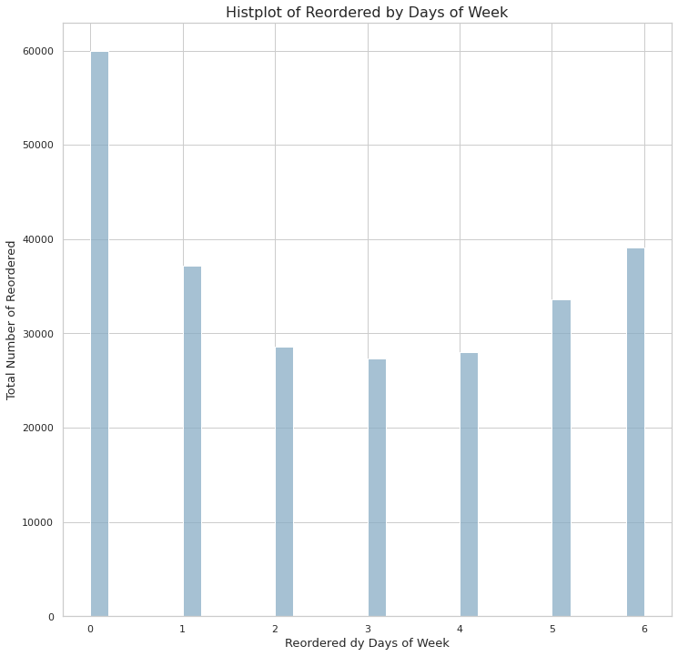

• 위의 테이블이 보여주는 값에 따르면 일주일 중 0, 1, 6에 가장 많은 소비가 이루어졌다.
• 현재 인덱스에 따른 요일 정보를 알 수 없기 때문에 우선 요일 0, 1, 6이라 칭하고 세개의 요일에 따른 재구매율을 확인하자.

3.4.1 전체 요일에 따른 재구매율

pd.crosstab(train['order_dow'], train['reordered'], normalize='index')

reordered 0 1
order_dow
0 0.389994 0.610006
1 0.400654 0.599346
2 0.407971 0.592029
3 0.409911 0.590089
4 0.400812 0.599188
5 0.388554 0.611446
6 0.402141 0.597859

• 요일에 따른 재주문율은 크게 다르지 않다.

3.5 주문 시간(order_hour_of_day)에 따른 재주문량

# histplot of total number of order by order_hour_of_day
plt.figure(figsize=(12,12))
ohd_hist = sns.histplot(x='order_hour_of_day',
                        bins=24,
                        data=train)
# xlab and ylab
ohd_hist.set_xlabel('Order Hour of Day', fontsize=13)
ohd_hist.set_ylabel('Total Number of Order', fontsize=13)
ohd_hist.set_title('Histplot of Ordered by Order Hour of Day', fontsize=16)
plt.show()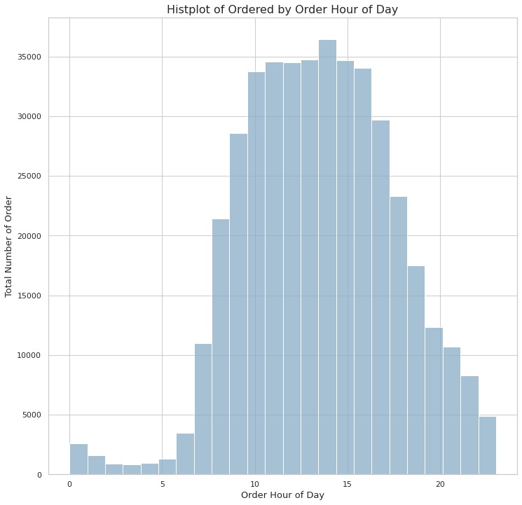

• Histplot에 따르면 10시 부터 17시 사이에 주문량이 가장 많다.

3.5.1 요일에 따른 시간별 주문량

day0 = train[train['order_dow']==0]
day1 = train[train['order_dow']==1]
day2 = train[train['order_dow']==2]
day3 = train[train['order_dow']==3]
day4 = train[train['order_dow']==4]
day5 = train[train['order_dow']==5]
day6 = train[train['order_dow']==6]

plt.figure(figsize=(18, 5)) ## plot에 대한  matplotlib 생성
## day0
plt.subplot(2,4,1)
day0_hist = sns.histplot(x='order_hour_of_day',bins=24,data=day0)
##day1
plt.subplot(2,4,2)
day1_hist = sns.histplot(x='order_hour_of_day',bins=24,data=day1)

## day2
plt.subplot(2,4,3)
day2_hist = sns.histplot(x='order_hour_of_day',bins=24,data=day2)

## day3
plt.subplot(2,4,4)
day3_hist = sns.histplot(x='order_hour_of_day',bins=24,data=day3)

## day4
plt.subplot(2,4,5)
day4_hist = sns.histplot(x='order_hour_of_day',bins=24,data=day4)

## day5
plt.subplot(2,4,6)
day5_hist = sns.histplot(x='order_hour_of_day',bins=24,data=day5)

## day6
plt.subplot(2,4,7)
day6_hist = sns.histplot(x='order_hour_of_day',bins=24,data=day6)

plt.show()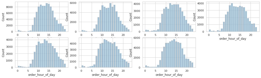

• 각 요일에서 시간별 총 주문량은 차이가 없어보인다.
• 요일별 재주문량을 살펴보자

plt.figure(figsize=(18, 5)) ## plot에 대한  matplotlib 생성
## day0
plt.subplot(2,4,1)
day0_hist = sns.histplot(x='order_hour_of_day',bins=24,data=day0[day0['reordered']==1])
##day1
plt.subplot(2,4,2)
day1_hist = sns.histplot(x='order_hour_of_day',bins=24,data=day1[day1['reordered']==1])

## day2
plt.subplot(2,4,3)
day2_hist = sns.histplot(x='order_hour_of_day',bins=24,data=day2[day2['reordered']==1])

## day3
plt.subplot(2,4,4)
day3_hist = sns.histplot(x='order_hour_of_day',bins=24,data=day3[day3['reordered']==1])

## day4
plt.subplot(2,4,5)
day4_hist = sns.histplot(x='order_hour_of_day',bins=24,data=day4[day4['reordered']==1])

## day5
plt.subplot(2,4,6)
day5_hist = sns.histplot(x='order_hour_of_day',bins=24,data=day5[day5['reordered']==1])

## day6
plt.subplot(2,4,7)
day6_hist = sns.histplot(x='order_hour_of_day',bins=24,data=day6[day6['reordered']==1])

plt.show()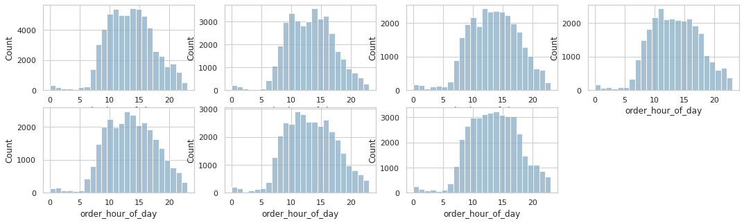

• 시간별 재주문량의 차이점도 크게 보이진 않는다.
• 즉 주문량이 많은 시간대엔 절대적인 재주문량 또한 절대적으로 높다.

  요일과 시간에 따라 재주문량이 영향을 받지 않는다.

4. EDA의 결과

• 재주문이 가장 많은 Department는 아래의 표와 같다.

4	16	19	7	1
Produce	Dairy eggs	Snacks	Beverages	Frozen

• 절대적으로 거래량이 많은건 Produce department이다.

• Monthly order 해택으로 인해 30일에 주문량과 재주문량이 가장 높은걸로 추측된다.

• 그러나 재구매율이 가장 높은건 일주일 단위로 이루어 진다.

• Monthly order해택보다 Weekly order에 대한 해택을 만들어 주는게 더 효율적일 것으로 추측된다.

• 가장 주문량과 재주문량이 많은 시간대는 요일에 상관없이 10~17시 사이이다.

• 10~17시 사이에 팝업 광고나 특별세일 등을 넣으면 효과적인 마케팅이 될것으로 추측된다.