1 Setting

1.1 Library Setting

from sklearn.impute import SimpleImputer
from IPython.display import display
import plotly.figure_factory as ff
import plotly.graph_objects as go
import seaborn as sns
import matplotlib.pyplot as plt
import numpy as np
import pandas as pd
import sklearn
from sklearn.experimental import enable_iterative_imputer
from sklearn.linear_model import LinearRegression
from sklearn.model_selection import StratifiedKFold
from sklearn.model_selection import train_test_split
from sklearn.metrics import roc_auc_score

1.2 Data Import

# import train & test data
train = pd.read_csv("../input/tabular-playground-series-sep-2021/train.csv")
test = pd.read_csv("../input/tabular-playground-series-sep-2021/test.csv")
sample = pd.read_csv("../input/tabular-playground-series-sep-2021/sample_solution.csv")

2 EDA

2.1 Skimming the Data Sets

train.head()

• 120 columns in train data

  The dataset includes 118 features and one target variable, 'claim'.

train.describe().T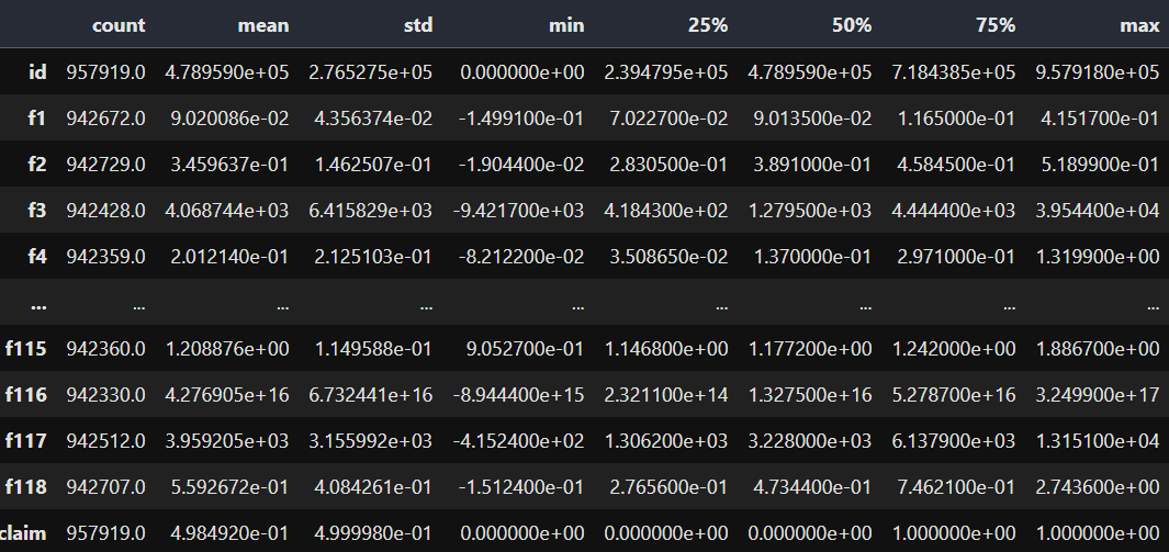

2.2 Cheacking the Missing Values

print(" train data")
print(f' Number of rows: {train.shape[0]}\n Number of columns: {train.shape[1]}\n No. of missing values: {sum(train.isna().sum())}')

train data
Number of rows: 957919
Number of columns: 120
No. of missing values: 1820782

print(" test data")
print(f' Number of rows: {test.shape[0]}\n Number of columns: {test.shape[1]}\n No. of missing values: {sum(test.isna().sum())}')

test data
Number of rows: 493474
Number of columns: 119
No. of missing values: 936218

• The training set has 1,820,782 missing values.
• The testing set has 936,218 missing values.

# number of misssing values by feature
print("number of misssing values by feature")
train.isnull().sum().sort_values(ascending = False)

number of misssing values by feature
f31 15678
f46 15633
f24 15630
f83 15627
f68 15619
...
f104 15198
f2 15190
f102 15168
id 0
claim 0
Length: 120, dtype: int64

# train_data missing values
null_values_train = []
for col in train.columns:
    c = train[col].isna().sum()
    pc = np.round((100 * (c)/len(train)), 2)            
    dict1 ={
        'Features' : col,
        'null_train (count)': c,
        'null_trian (%)': '{}%'.format(pc)
    }
    null_values_train.append(dict1)
DF1 = pd.DataFrame(null_values_train, index=None).sort_values(by='null_train (count)',ascending=False)


# test_data missing values
null_values_test = []
for col in test.columns:
    c = test[col].isna().sum()
    pc = np.round((100 * (c)/len(test)), 2)            
    dict2 ={
        'Features' : col,
        'null_test (count)': c,
        'null_test (%)': '{}%'.format(pc)
    }
    null_values_test.append(dict2)
DF2 = pd.DataFrame(null_values_test, index=None).sort_values(by='null_test (count)',ascending=False)


df = pd.concat([DF1, DF2], axis=1)
df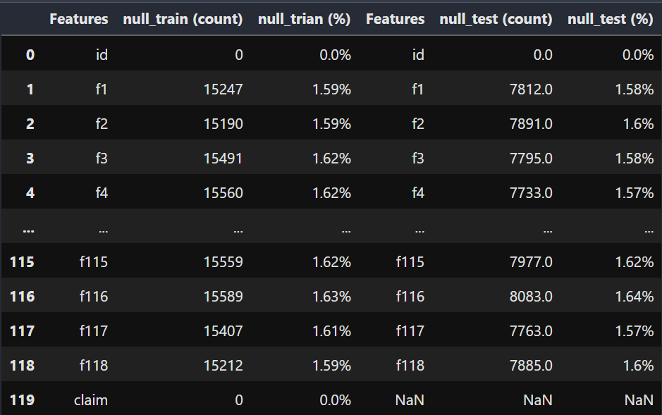

• It seems like every feature has approximatley same number of missing values.

df = pd.DataFrame()
df["n_missing"] = train.drop(["id", "claim"], axis=1).isna().sum(axis=1)
df["claim"] = train["claim"].copy()

fig, ax = plt.subplots(figsize=(12,5))
ax.hist(df[df["claim"]==0]["n_missing"],
        bins=10, edgecolor="black",
        color="darkseagreen", alpha=0.7, label="claim is 0")
ax.hist(df[df["claim"]==1]["n_missing"],
        bins=10, edgecolor="black",
        color="darkorange", alpha=0.7, label="claim is 1")
ax.set_title("Missing Values Distributionin in Each Target Class", fontsize=20, pad=15)
ax.set_xlabel("Missing Values Per Row", fontsize=14, labelpad=10)
ax.set_ylabel("Number of Rows", fontsize=14, labelpad=10)
ax.legend(fontsize=14)
plt.show()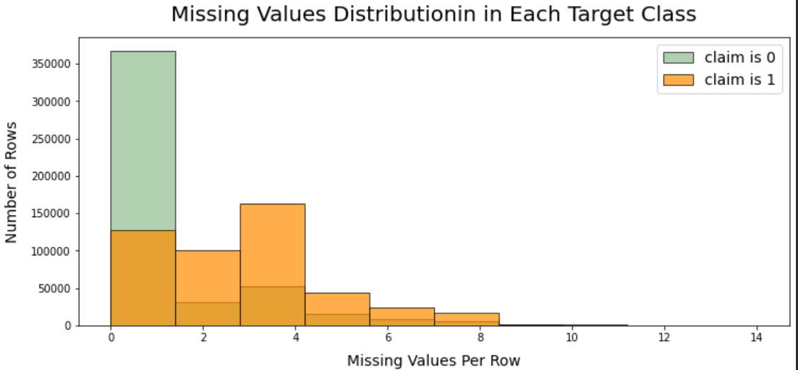

• The plot shows that the rows have missing values and claim = 0 is skewed to the first few rows.
• The rows have missing values and claim = 1 are more likely distributed then claim = 0.

# looking at Claim column
fig, ax = plt.subplots(figsize=(6, 6))

bars = ax.bar(train["claim"].value_counts().index,
              train["claim"].value_counts().values,              
              edgecolor="black",
              width=0.4)
ax.set_title("Claim (target) values distribution", fontsize=20, pad=15)
ax.set_ylabel("Amount of values", fontsize=14, labelpad=15)
ax.set_xlabel("Claim (target) value", fontsize=14, labelpad=10)
ax.set_xticks(train["claim"].value_counts().index)
ax.tick_params(axis="both", labelsize=14)
ax.bar_label(bars, [f"{x:2.2f}%" for x in train["claim"].value_counts().values/(len(train)/100)],
                 padding=5, fontsize=15)
ax.bar_label(bars, [f"{x:2d}" for x in train["claim"].value_counts().values],
                 padding=-30, fontsize=15)
ax.margins(0.2, 0.12)
ax.grid(axis="y")

plt.show()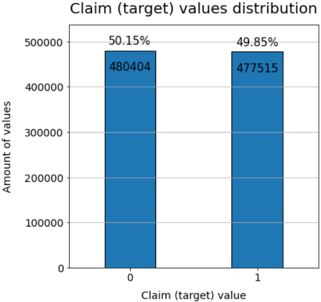

• Before the NaN-values are dropped, 'claim' = 0 and 1 have approximately have same number of rows.

# proportion of no null in each row
train1 = train[train.isna().sum(axis=1)==0]
print("proportion of no null data : %.2f" %(len(train1)/len(train)*100))
print("number of claim 1 in no null data : %d" %(len(train1[train1['claim']==0])))
print("number of claim 0 in no null data : %d" %(len(train1[train1['claim']==1])))

proportion of no null data : 37.53
number of claim 1 in no null data : 310909
number of claim 0 in no null data : 48555

fig, ax = plt.subplots(figsize=(6, 6))

bars = ax.bar(train1["claim"].value_counts().index,
              train1["claim"].value_counts().values,              
              edgecolor="black",
              width=0.4)
ax.set_title("Claim (target) values distribution", fontsize=20, pad=15)
ax.set_ylabel("Amount of values", fontsize=14, labelpad=15)
ax.set_xlabel("Claim (target) value", fontsize=14, labelpad=10)
ax.set_xticks(train1["claim"].value_counts().index)
ax.tick_params(axis="both", labelsize=14)
ax.bar_label(bars, [f"{x:2.2f}%" for x in train1["claim"].value_counts().values/(len(train1)/100)],
                 padding=5, fontsize=15)
ax.bar_label(bars, [f"{x:2d}" for x in train1["claim"].value_counts().values],
                 padding=-30, fontsize=15)
ax.margins(0.2, 0.12)
ax.grid(axis="y")

plt.show()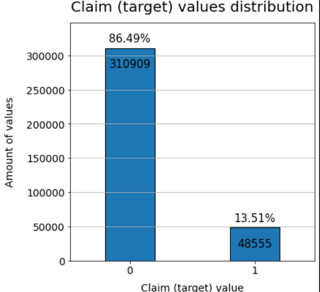

• However, if Nan-values are dropped, then proportion of 'claim' = 0 and 1 are vary different.
• The plot tells most of missing values are located in rows where 'claim' = 1.
• Thus, it will be inbalanced if the Nan-values are simply dropped.

2.3 Cheacking the Distribution of Features.

target = train.pop('claim')

train_ = train[0:9579]
test_ = test[0:4934]

# distribution of Features f1 to f60
L = len(train.columns[0:60])
nrow= int(np.ceil(L/6))
ncol= 6

remove_last= (nrow * ncol) - L

fig, ax = plt.subplots(nrow, ncol,figsize=(24, 30))
#ax.flat[-remove_last].set_visible(False)
fig.subplots_adjust(top=0.95)
i = 1
for feature in train.columns[0:60]:
    plt.subplot(nrow, ncol, i)
    ax = sns.kdeplot(train_[feature], shade=True, color='cyan',  alpha=0.5, label='train')
    ax = sns.kdeplot(test_[feature], shade=True, color='darkblue',  alpha=0.5, label='test')
    plt.xlabel(feature, fontsize=9)
    plt.legend()
    i += 1
plt.suptitle('DistPlot: train & test data', fontsize=20)
plt.show()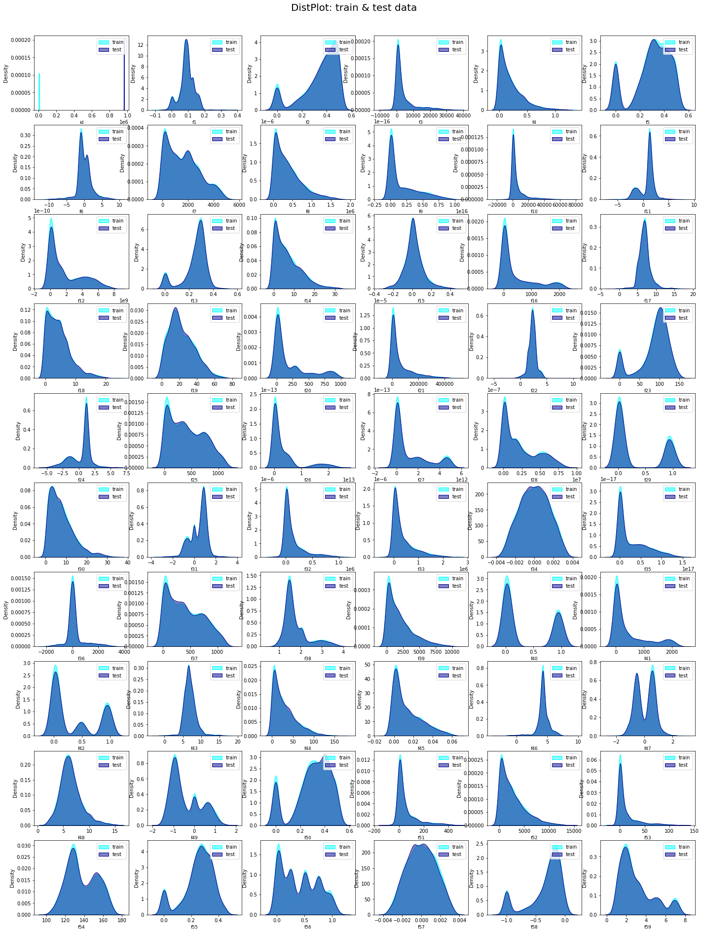

# distribution of Features f61 to f118
L = len(train.columns[60:])
nrow= int(np.ceil(L/6))
ncol= 6

remove_last= (nrow * ncol) - L

fig, ax = plt.subplots(nrow, ncol,figsize=(24, 30))
#ax.flat[-remove_last].set_visible(False)
fig.subplots_adjust(top=0.95)
i = 1
for feature in train.columns[60:]:
    plt.subplot(nrow, ncol, i)
    ax = sns.kdeplot(train_[feature], shade=True, color='cyan',  alpha=0.5, label='train')
    ax = sns.kdeplot(test_[feature], shade=True, color='darkblue',  alpha=0.5, label='test')
    plt.xlabel(feature, fontsize=9)
    plt.legend()
    i += 1
plt.suptitle('DistPlot: train & test data', fontsize=20)
plt.show()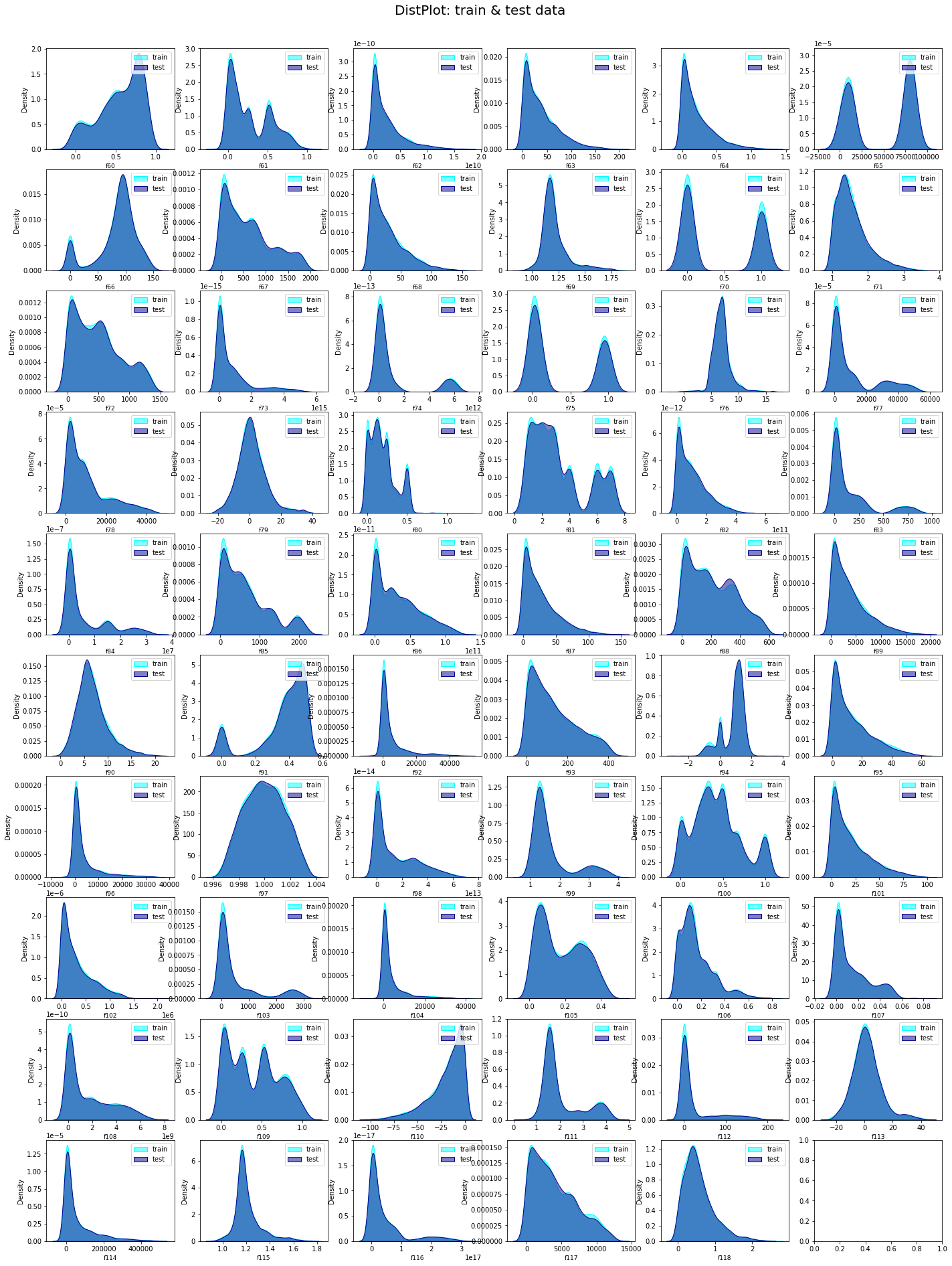

2.4 Cheacking the Box-plots

# outlier of train data
df_plot = ((train - train.min())/(train.max() - train.min()))
fig, ax = plt.subplots(4, 1, figsize = (25,25))
sns.boxplot(data = df_plot.iloc[:, 1:30], ax = ax[0])
sns.boxplot(data = df_plot.iloc[:, 30:60], ax = ax[1])
sns.boxplot(data = df_plot.iloc[:, 60:90], ax = ax[2])
sns.boxplot(data = df_plot.iloc[:, 90:120], ax = ax[3])

# outlier of test data
df_plot = ((test - test.min())/(test.max() - test.min()))
fig, ax = plt.subplots(4, 1, figsize = (25,25))
sns.boxplot(data = df_plot.iloc[:, 1:30], ax = ax[0])
sns.boxplot(data = df_plot.iloc[:, 30:60], ax = ax[1])
sns.boxplot(data = df_plot.iloc[:, 60:90], ax = ax[2])
sns.boxplot(data = df_plot.iloc[:, 90:119], ax = ax[3])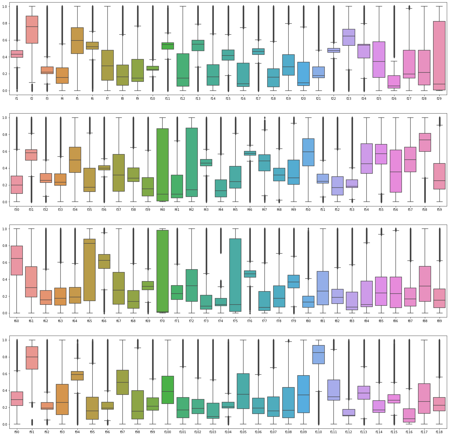

• Boxplots show that both training and testing sets are similarly distributed.

# correlation of train
corr = train.corr()
mask = np.triu(np.ones_like(corr, dtype = bool))

plt.figure(figsize = (15, 15))
plt.title('Corelation matrix')
sns.heatmap(corr, mask = mask, cmap = 'Spectral_r', linewidths = .5)

plt.show()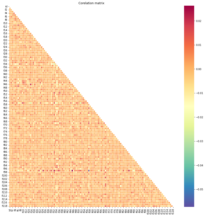

# correlation of train
corr = test.corr()
mask = np.triu(np.ones_like(corr, dtype = bool))

plt.figure(figsize = (15, 15))
plt.title('Corelation matrix')
sns.heatmap(corr, mask = mask, cmap = 'Spectral_r', linewidths = .5)

plt.show()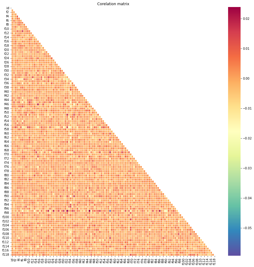

• The correlation between the two data are also similar.
• Overall, every feature in both training and testing sets are vary similar.