Bayesian Estimation (1) : Conjugate prior & Variational Inference

bayesian estimation은 어떠한 모수(Parameter)가 unknown constant가 아닌, 어떠한 확률 분포를 가지는 확률 변수라고 가정한다. 이러한 가정을 바탕으로 데이터 $\mathbf{x}$가 주어졌을 때, 모수 $\theta$의 확률 분포인 $p(\theta | \mathbf{x})$를 구하거나 근사하는 것이 베이즈 추정의 목적이다. 가능도 $L(\theta)$를 최대화하는 모수를 찾는 maximum likelihood estimation과는 다르다.

베이즈 추정을 하기 위해서는 사전 분포(prior)라는 개념에 대해 이해해야 한다. prior란, 어떠한 데이터가 주어지기에 앞서 우리가 모수 $\theta$에 대해 가지는 믿음이다.

예를 들어, $\mathbf{Bernoulli}(\theta)$의 모수인 $\theta$의 분포를 추정한다고 해 보자. 이 때, $\theta$는 0과 1 사이의 값이고 우리는 $p(\theta) \sim \mathbf{Uniform}(0,1)$ 이라고 가정할 수 있다. 이와 같이, 데이터를 보기에 앞서 모수가 따르는 분포에 대한 가정이 prior이다. 어떤 Prior distribution을 선택하느냐에 따라, 최종적으로 구하고자 하는 $p(\theta|\mathbf{x})$가 닫힌 형식으로 구해지기도 하고, 그렇지 않기도 한다.

베이즈 추정의 목적은 prior로부터 시작해서, 데이터가 주어졌을 때의 사후분포(posterior)인 $p(\theta|\mathbf{x})$를 구하는 것이다.

우리가 구하고자 하는 $p(\theta|\mathbf{x})$는 베이즈 정리에 따라 아래와 같이 표현될 수 있다.

$p(\theta|\mathbf{x}) ={{p(\mathbf{x}|\theta)p(\theta)}\over{p(\mathbf{x})}} ={{p(\mathbf{x}|\theta)p(\theta)}\over{\int p(\mathbf{x}|\theta)p(\theta)d\theta}}$

해당 수식에서 분자는 likelihood와 prior의 곱이므로 쉽게 구할 수 있지만, 분모는 경우에 따라 부정적분을 구하기 난해(intractable)할 수도 있다. 이런 경우에는 닫힌 형태의 해를 구할 수 없고, 근사적인 방법에 의존해야 한다.

베이즈 추정을 하기 위한 방법이 크게 세 가지가 있다.

• Conjugate Prior
• Variational Inference
• Markov Chain Monte Carlo(MCMC)

이번 포스팅에서는 conjugate prior와 variational inference에 대해 간략히 소개해보고자 한다. 이 중, variational inference는 비교적 최근 연구인 VAE(Variational Autoencoding Bayes)에서도 활용된 개념이다.

1. Conjugate Prior

데이터가 어떤 분포를 따를 때, prior를 특정 분포로 설정하면, posterior 또한 prior와 같은 족의 분포로 구해지는 경우가 있다. 예시를 들면 아래와 같다.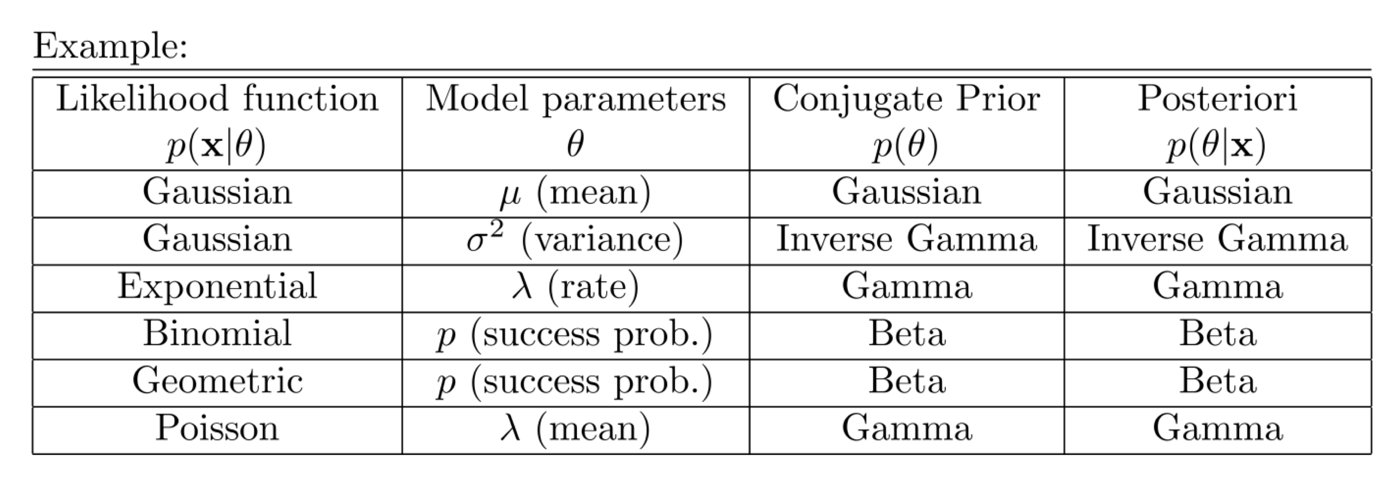

데이터가 정규 분포를 따른다고 가정했을 때, $\mu$가 정규분포를 따른다고 가정하면, $p(\mu|\mathbf{x})$도 정규분포를 따름을 수학적으로 유도할 수 있다. 유도 과정은 아래와 같다.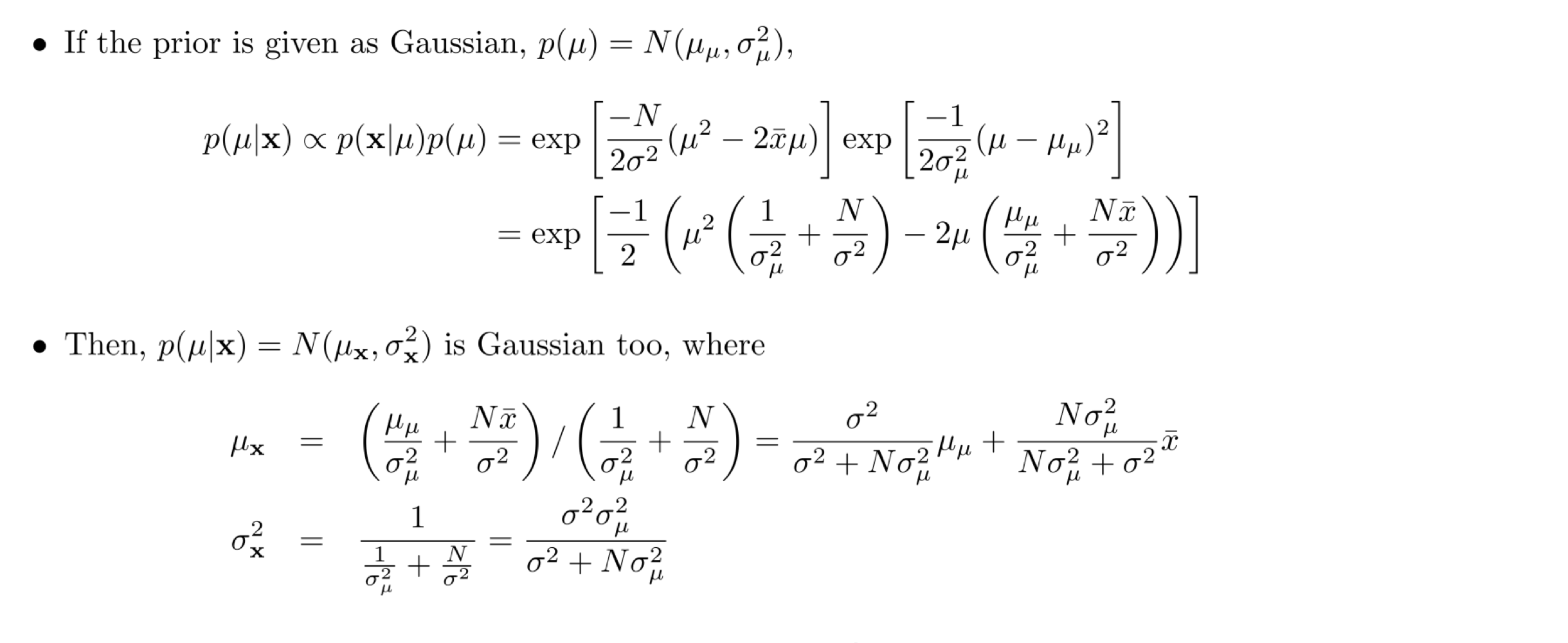

위와 같이, 다양한 분포들에 대해 posterior를 일반적으로 구해 보았다.

• $p(\sigma^2|x)\sim IGamma(\alpha+{n/2}, \beta+n\bar{x}/2-n\mu/2)$ where $\sigma^2\sim IGamma(\alpha, \beta)$ and $X \sim N(\mu, \sigma^2)$
• $p(\lambda|x)\sim Gamma(n+\alpha, n\bar{x}+\beta)$ where $\lambda\sim Gamma(\alpha, \beta)$ and $X \sim \mathbf{Exp}(\lambda)$
• $p(\theta|x)\sim Beta(\alpha+n\bar{x}, nk+\beta-n\bar{x})$ where $\theta \sim Beta(\alpha, \beta)$ and $X \sim Binomial(k,\theta)$
• $p(\theta|x)\sim Beta(\alpha+n\bar{x}, \beta + n)$ where $\theta \sim Beta(\alpha, \beta)$ and $X \sim Geo(\theta)$
• $p(\lambda|x) \sim Gamma(\alpha+n\bar{x}, \beta + n)$ where $\lambda \sim Gamma(\alpha, \beta)$ and $X \sim Poisson(\lambda)$

2. Variational Inference

변분추론(Variational Inference)는 posterior distribution을 closed form으로 구할 수 없을 때 즉,
$p(\theta|\mathbf{x}) ={{p(\mathbf{x}|\theta)p(\theta)}\over{p(\mathbf{x})}} ={{p(\mathbf{x}|\theta)p(\theta)}\over{\int p(\mathbf{x}|\theta)p(\theta)d\theta}}$ 의 분모에 대한 적분이 intractable할 때 사용하는 방식이다. 우리는 모수에 대한 prior와 data distribution을 가정하기 때문에, $p(\theta)$와 $p(x|\theta)$는 tractable하다. 하지만, 분모의 $p(x)$를 구하는 과정이 intractable하면, variational inference를 통해 최적의 posterior를 근사해야 한다.

variational inference의 목적은 $w$로 parameterized 된 $q_{w}(\theta|x)$라는 함수가, true posterior인 $p(\theta|x)$와 가장 가까워지도록 $w$를 최적화 하는 것이다.

여기서 $q_{w}(\theta|x)$를 Posterior를 근사하기 위한 특정 분포의 확률밀도함수 그 자체로 이해하면, $w$는 해당 분포의 모수로 볼 수 있다. 반면 딥러닝의 관점에서 $w$는, $q_{w}(\theta|x)$ 분포의 모수를 추정하는 weight를 의미하기도 한다.

아래 수식을 보자.

$\mathcal{F}(w) = \mathbb{E}_{q_{w}(\theta|x)}[\ln {{q_{w}(\theta|x)}\over{p(x|\theta)p(\theta)}}] = \int q_{w}(\theta|x) \ln {{q_{w}(\theta|x)}\over{p(x|\theta)p(\theta)}} = \int q_{w}(\theta|x) \ln {{q_{w}(\theta|x)}\over{p(\theta|x)p(x)}} = D_{KL}(q_{w}(\theta|x) | p(\theta|x)) - \ln p(x)$

이 수식에서 $\mathcal{F}(w)$를 minimization objective라고 이해하면 된다. 계산이 tractable한 $\mathcal{F}(w)$를 $w$에 대해 최소화하는 것은 결국 $q_{w}(\theta|x)$ 와 $p(\theta|x)$간의 KL Divergence를 최소화하는 것과 상응한다.