Github

Papers

Learning Audio-Visual Speech Representation by Masked Multimodal Cluster Prediction, in Proc. ICLR 2022

Robust Self-Supervised Audio-Visual Speech Recognition, in Proc. Interspeech 2022 (blog)

Learning Lip-Based Audio-Visual Speaker Embeddings with AV-HuBERT, in Proc. Interspeech 2022

Practice of the Conformer Enhanced Audio-Visual Hubert on Mandarin and English, in Proc. ICASSP 2023

Overview: Hubert

• Published on arXiv on: 14 Jun 2021 by: FAIR
  

Pre-training

• HuBERT pre-training is very similar to BERT
  • Mask some of the input tokens and train the model to retrieve these missing/masked tokens
    • One key challenge for HuBERT is that speech is continuous, unlike text which is discrete.
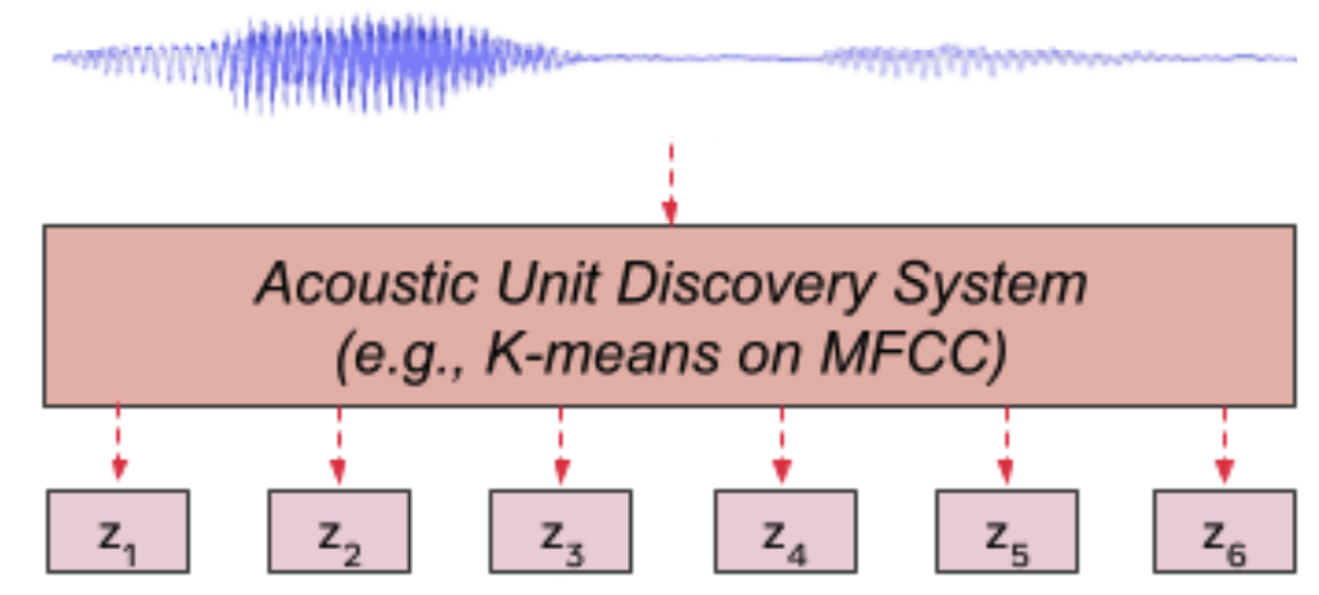
    • To overcome this challenge, Acoustic Unit Discover System was used (as shown in the following figure)
      • to cluster continuous input speech into discrete units (or codebooks) that can be masked while pre-training

Acoustic Unit Discovery System

• Let $X = \left\lbrack x_{1},\ …x_{T} \right\rbrack$ denote a speech utterance of $T$ frames, the acoustic unit discovery system uses a clustering algorithm (e.g k-means) on this input features $X$ to cluster them into a predefined number of clusters $C$
• The discovered hidden units are denoted with $Z = \left\lbrack z_{1},\ …z_{T} \right\rbrack$ where $z_{t} \in \lbrack C\rbrack$ as shown in the following figure

• To improve the clustering quality, they tried two different methods:
  • Cluster Ensembles:
    • An ensemble of clusters can provide complementary information to facilitate representation learning.
    • For example, an ensemble of k-means models with different codebook sizes can create targets of different classes (vowel/consonant).
  • Iterative Refinement of Cluster Assignments:
    • A new generation of clusters can be created using the pre-trained model from the earlier generation.

HuBERT Model

HuBERT follows the same architecture as wav2vec 2.0 with two different parts:

• CNN Encoder:

  The convolutional waveform encoder generates a feature sequence at a 20ms framerate for audio sampled at 16kHz (CNN encoder down-sampling factor is 320x).

  The audio encoded features are then randomly masked.
  

• BERT:

  The encoded features from the CNN Encoder get masked and sent to this model which can be considered as an acoustic BERT.

  Regarding masking, they used the same strategy used for SpanBERT 

  where p% of the timesteps are randomly selected as start indices

  And then BERT learns to predict the latent features of the unmasked and the masked input equally.

Objective

HuBERT is pre-trained to minimize the cross-entropy loss computed over masked and unmasked timesteps as $\mathcal{L}_m$ and $\mathcal{L}_u$ respectively.

The final loss is computed as a weighted sum of the two terms with a hyper-parameter $\alpha$

• Where $A$ is the projection matrix appended at the end of HuBERT during
  pre-training;
  - a different projection matrix is used for different cluster model.
• $e_{c}$ is the embedding for code-word $c$
• $sim(.,\ .)$ computes the cosine similarity between two vectors
• $\tau$ scales the logit, which is set to $0.1$

💡 **Note:** After pre-training and during fine-tuning, the projection layer(s) is removed and replaced with a randomly initialized Softmax layer

AV-HuBERT

Audio-Visual HuBERT

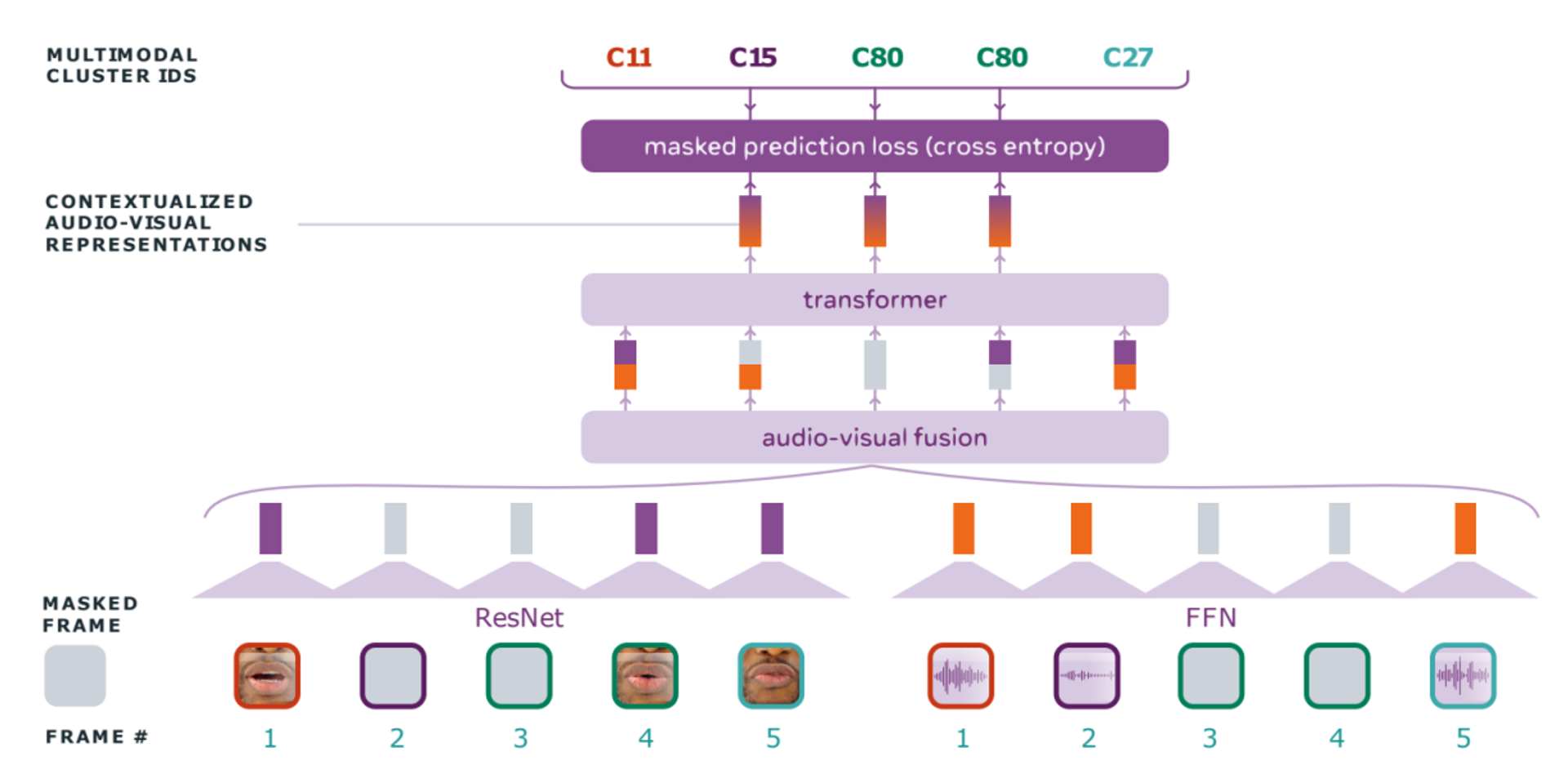
The AV-HuBERT model is a multimodal learning approach that integrates both acoustic and visual frames for training

It uses light-weight encoders specific to each modality to generate intermediate features.

Audio-visual input

• AV-HuBERT is a model that combines audio features with the visual features
• More formally, given an audio stream $A = \left\lbrack a_{1},\ …a_{T} \right\rbrack$ and a visual stream $I = \left\lbrack i_{1},\ …i_{T} \right\rbrack$ aligned together

Masking

• Both the input audio stream $A$ and the image stream $I$ are going to be masked independently using two different masking probabilities $m_{a}$ and $m_{v}$

  • That’s because inferring the masked targets given the audio stream is more straightforward than using the visual stream stream

    💡 So, setting a high masking probability for acoustic frames is essential to help the whole model capture the language characteristics
    💡 On the contrary, setting a high masking probability for the visual input hurts its ability to learn meaningful features

• The audio stream $A$ will be masked into $\widetilde{A}$ by a binary masking $M$.

  • Specifically, $\forall t \in M, a_{t}$ is replaced with a masked embedding following the same masking method as HuBERT

  • In parallel, the input image stream $I$ will be masked into $\widetilde{I}$ by a novel masking strategy

    Masking by substitution

    • some segments in the visual stream will be substituted with random segments from the same video
    • More formally, given an input video $I = \left\lbrack i_{1},\ …i_{T} \right\rbrack$, an imposter segment $J = \left\lbrack j_{1},\ …j_{\mathcal{T}} \right\rbrack$ taken from the original video will be used to corrupt the input video to $\widetilde{I}$
      1. masking $n$ intervals $M = \left\{ \left( s_i, t_i \right) \right\}_{1 \leq i \leq n}$
      2. replacing them with the imposter video $J$ using an offset integer $p_i$ sampled from the interval $\left\lbrack 0,\ \mathcal{T} - (t_i - s_i) \right\rbrack$, as shown in the following formula:
      ${\widetilde{I}}_{\left( s_{i}:t_{i} \right)} = J_{\left( p_{i}:p_{i} + t_{i} - s_{i} \right)},\ \ \forall 1 \leq i \leq n$

    💡 To solve the task, the model needs to first identify the fake frames and then infer the labels belonging to the original frames

    💡 the fake segment detection sub-task becomes less trivial compared to when using vanilla masking or substitution with non-consecutive frames.

• Model

  • audio encoder

    • a simple Fully-Forward Network (FFN) will be used to extract acoustic features $F^{(a)} = \left\lbrack f_{1}^{(a)},\ …f_{T}^{(a)} \right\rbrack$from the masked audio stream $\widetilde{A}$

  • visual encoder

    • modified ResNet-18, will be used to extract visual features $F^{(v)} = \left\lbrack f_{1}^{(v)},\ …f_{T}^{(v)} \right\rbrack$ from the visual stream $\widetilde{I}$

  • Then, these acoustic features $F^{(a)}$ will be concatenated with the visual features $F^{(v)}$
    - on the channel-dimension forming audio-visual features $F^{(av)}$
    - according to two random probabilities $p_{m}$ and $p_{a}$ useful for modality dropout

    

  • transformer encoder

    • Then, the acoustic-visual features are encoded into a sequence of contextualized features $E = \left\lbrack e_{1},\ …e_{T} \right\rbrack$
    • followed by a linear projection layer which maps features into logits:

• Finally, AV-HuBERT is pre-trained to first identify the fake frames and then infer the labels belonging to the original frames according to the following loss function:
  $\mathcal{L} = - \sum_{t \in M^{(a)} \cup M^{(v)}}^{}{\log\left( p_{t}.z_{t} \right)} - \alpha\sum_{t \notin M^{(a)} \cup M^{(v)}}^{}{\log\left( p_{t}.z_{t} \right)}$
  • Where $Z = \left\lbrack z_{1},\ …z_{T} \right\rbrack$ is the clustered representations using clustering algorithm (e.g. k-means) such that each $z_{t}$ belongs to one of $V$ different clusters (codebooks).
    $z_{t} = kmeans\left( h_{t} \right),\ \ \ \ \ z_{t} \in \left\{ 1,\ 2,\ ...V \right\}$
    • The input features $h_{t}$ to the clustering algorithm change based on the training iteration
      • For the first iteration, MFCC acoustic features extracted from the input audio stream $A$ are used.
      • For the other iterations, intermediate layers of the Visual HuBERT model are used.

Experiment

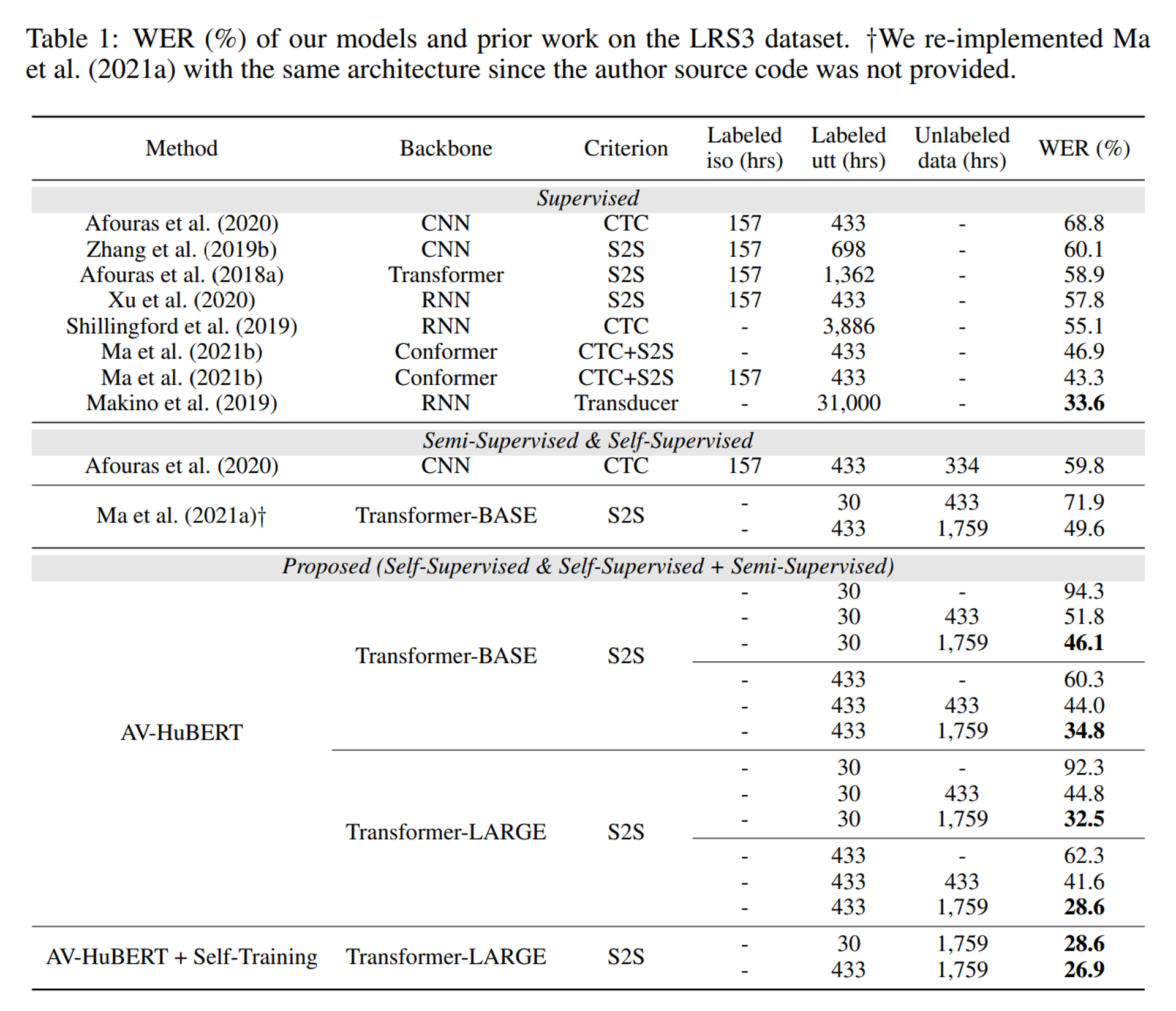
Lip Reading

Speech Recognition (AVSR)

Reference blog

• https://anwarvic.github.io/speech-recognition/HuBERT
  https://anwarvic.github.io/speech-recognition/AV-HuBERT_for_AVSR