• “From simulated mixtures to simulated conversations as training data for end-to-end neural diarization” , in Proc. Interspeech, 2022. (BUT) [Paper] [Code]

• "Multi-Speaker and Wide-Band Simulated Conversations as Training Data for End-to-End Neural Diarization", in Proc. ICASSP, 2023. (BUT) [Paper] [Code]

Problem

• EEND require large amounts of annotated data for training but available annotated data are scarce
• EEND works have used mostly simulated mixtures for training [Ref Blog]
  • little analysis has been presented
    • about how the simulations were devised nor what impact have the used augmentations
  • simulated mixtures do not resemble real conversations in many aspects
    • specially when more than two speakers are included
• creating synthetic data becomes more challenging since the mismatch between (artificial) training and (authentic) test data can become much larger

Proposal

• alternative method for creating synthetic conversations
  • resemble real ones by using statistics about distributions of pauses and overlaps estimated on genuine conversations.

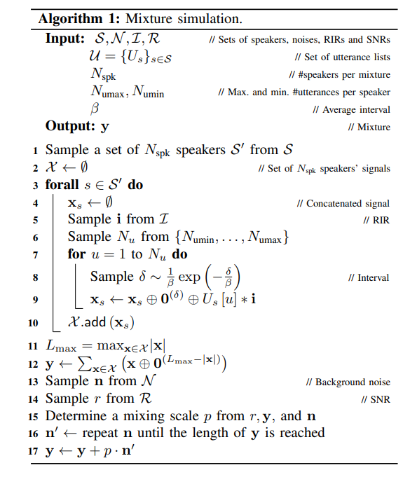
Simulated Mixture (SM)

1. Start with a group of speakers, each having their own unique spoken parts.
2. Randomly pick some speakers.
3. For each picked speaker, choose a part of their speech and add pauses to mimic natural conversation.
4. Each speaker's speech with pauses forms a unique sound channel.
5. Do this for all picked speakers, then mix these channels into one sound.
6. Add extra sounds like background noise to make it more realistic.
7. Depending on the pause length used, there could be a lot of overlapping speech

💡Please note that Yusuke et al. have referred as “utterances” to the segments of speech in a real conversation.
But on this paper
The utterances: complete phrases or sentences that the speakers have said
The segments: portions of speech from the speakers (defined by the VAD labels)

Simulated Conversation (SC)

• aim to be more like real conversations than the Speaker Mixture (SM) method.

1. The SC method uses the full speech of each chosen speaker only once, not just parts like the old method.
2. The SC method mixes speakers' speech parts while keeping their order, but changes the order of when speakers take their turn.
3. Uses statistics from real conversations to determine pauses and overlaps.

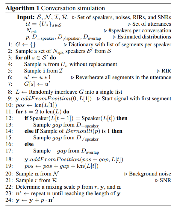
1. Initialize an empty dictionary G to store the list of segments for each speaker.
2. Randomly select a number of speakers (Nspk) from the total pool of speakers (S).
3. For each selected speaker:
   • Choose an utterance from the speaker's pool without replacement.
   • Select a Room Impulse Response (RIR).
   • Apply this RIR to all segments in the utterance to simulate reverberation.
   • Store the reverberated segments in the dictionary G.
4. Randomly interleave all speakers' segments stored in G into a single list (L).
   1. guaranteeing that the per-speaker order is kept while assigning random order to the speaker turns of the different speaker
5. Start the output signal (y) with the first segment from list L.
6. Initialize a position marker (pos) to the length of the first segment.
7. For each remaining segment in list L:
   • If the current segment and the previous segment are from the same speaker,
     • sample a +gap (pause) from the distribution of within-speaker pauses (D=speaker).
   • If a Bernoulli trial with probability p is successful,
     • sample a +gap (pause) from the distribution of between-speaker pauses (D!=speaker).
     • $p=\frac{ds}{ds+ov}, ds=\text{number of pauses}, ov=\text{number of overlaps}$
   • Otherwise,
     • sample a -gap (overlap) from the distribution of between-speaker overlaps (D_overlap).
   • Add the current segment to the output signal (y) at the position determined by the current marker (pos) plus the gap.
   • Update the position marker (pos) by adding the gap and the length of the current segment.
8. Select a background noise (n) from the pool of noises (N).
9. Select a signal-to-noise ratio (r) from the pool of SNRs (R).
10. Determine a mixing scale (p) from the selected SNR (r), the current output signal (y), and the selected noise (n).
11. Repeat the selected noise (n) until it matches the length of the signal, and add it to the output signal (y) at the mixing scale (p).

💡 utterance is not used more than once

In practice, the code is prepared to run until exhausting all utterances and re-start again until a given amount of times is reached or until generating a specific amount of audio

Ex. Radom Interaleaving
Speaker A said "Hello, how are you?" ⇒ "Hello," "how are you?"
Speaker B said "I'm fine, thank you," ⇒ "I'm fine," "thank you"

Interleaving might result
⇒ ["Hello," "I'm fine," "how are you?", "thank you"]
💡 Note that the order of each speaker's segments remains intact

• "Hello" always comes before "how are you?" for Speaker A
• "I'm fine" always comes before "thank you" for Speaker B
• but the speakers' turns are randomly ordered.

Experiments

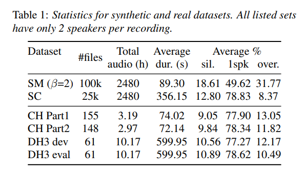
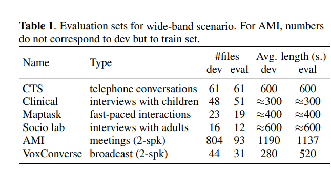
Real Dataset Statistics

💡 Results on CH, VoxConverse for evaluation with a forgiveness collar of 0.25s
💡 while the other sets mentioned above were scored with forgiveness collar 0s.

• Reducing the dependence on the fine-tuning stage

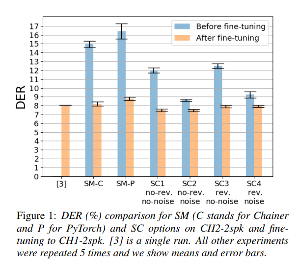
Comparsion on 2-Speaker

CH2-2spk

Augmentation

• adding background noises yielded significant gains. (SC2)
• Reverberating (SC3) the signals did not yield better results, suggesting that this might be more useful in scenarios where speakers don't have specific microphones, such as meetings or interviews.

💡 They noted that the choice of room impulse responses (RIRs) could be more narrowly selected to match real application scenarios, and that these aspects should be further studied

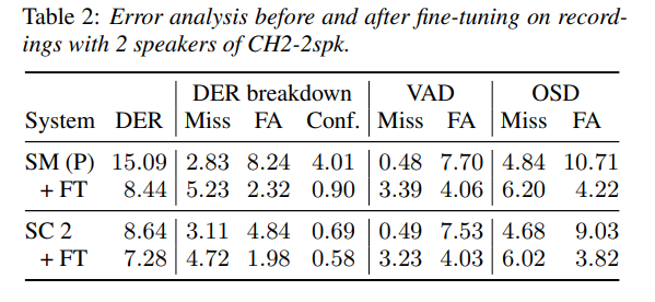
DER break down

• similarly in terms of VAD before and after fine-tuning.
• more significant differences were observed in terms of OSD
  • fewer false alarms for OSD, especially before fine-tuning
  • attributed to the higher percentage of overlap seen in SM.

💡 Mechanisms for favoring slightly higher percentages of overlap when creating SC are left for future studies

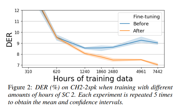
Amount of data analysis

• Performance degraded significantly when using only 310 hours of training data
• However, using 1240 hours of data (half the amount used in other experiments) resulted in similar performance
• More training data allowed the fine-tuned model to reach lower DER (about 7%)

CH2-2spk / DH3

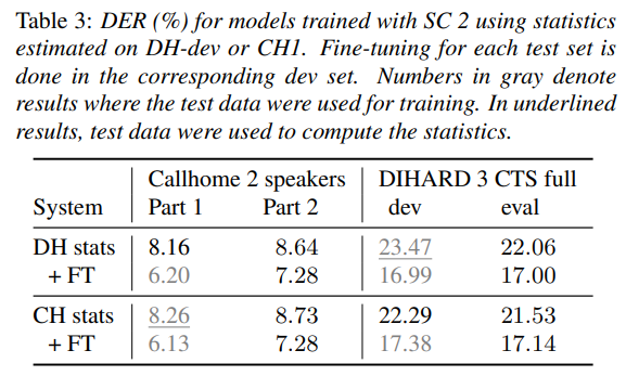
Eeffect of statistics source

• observed that it doesn't significantly impact performance

Comparison with Other Model (EEND-EDA)

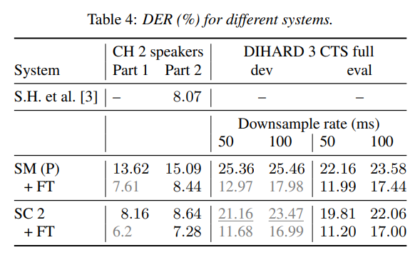
• Training with SC data yielded similar performance to training with SM after fine-tuning on Callhome.
• The impact of fine-tuning was more significant in the case of DIHARD CTS

  • One critical factor considered was the downsampling of the input data to produce one output every 100 ms.

  • This impacted results when evaluated with a 0s forgiveness collar, as in DIHARD.

    When evaluating at the standard downsampling of one output every 100 ms and 50 ms, a considerable error reduction was achieved after fine-tuning.

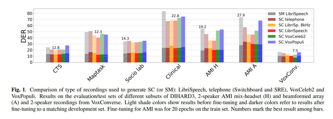
Comparison on Wide-band Scenario

• While differences between SM and SC performance were noticeable before fine-tuning, these differences reduced after the fine-tuning process

• Certain trends were observed: 8 kHz models performed the worst for Maptask and AMI sets,

  • suggesting higher frequencies are more relevant for these sets
  • ❓However, SC LibriSp. 8kHz is not degraded…?

• Models using VoxCeleb2 recordings showed better performance on VoxConverse due to similarities between these sets.

• SC outperformed in telephony scenarios (CTS), but in wide-band scenarios, fine-tuning played a significant role and Synthetic Mixtures (SM) yielded similar performance.

💡 Finetuning still plays a major role
💡 The key challenges lie not in the realism of the synthetic data, but in differences between the source and test data, quality of speaker annotation, and the conversationality.

• Tried generating SC using different statistics about pauses and overlaps from real conversations but found no significant differences

💡 Even though this research doesn't prove that better synthetic data can't be made for improved results without extra fine-tuning, the authors want to share the work to show what already tried in this field

• other areas for potential improvement like more realistic data augmentation techniques including background noises, reverberation, or loudness levels that match the application scenarios.

Multi-speaker experiments

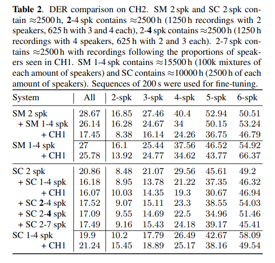
Different datasets were used for training, adapting (increasing speaker count), and fine-tuning the models.

• The performance when SC was used was considerably better than with SM.

• Adapting to more speakers significantly improved the performance, reducing the dependence on the fine-tuning step.

• Training on a dataset with a higher proportion of 4-speaker recordings improved the model's ability to handle more speakers.

• However, training with a dataset that mirrored the speaker proportions in the evaluation set (CH1) didn't show significant gains.

  • The research suggests that training sets might need to be larger to effectively learn to handle more speakers.

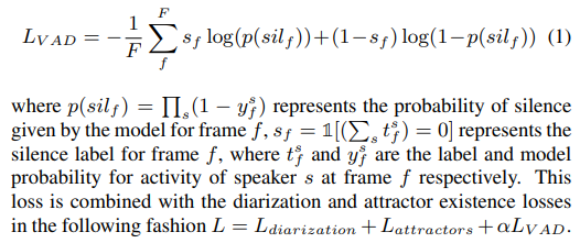
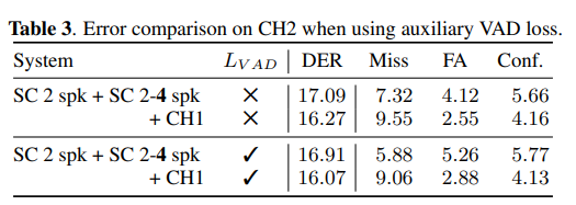
Auxiliary VAD Loss

• An additional VAD loss ($\alpha=0.2$) was also introduced in the adaptation stage, which allowed the model to more evenly balance missed and false alarm speech.
  • This resulted in better fine-tuning performance, comparable to that achieved when using the larger 1-4 speaker set.

💡The results hint that producing training data on-the-fly to encourage larger variability might be beneficial.