본 포스트는 [모두를 위한 딥러닝 시즌2] 강의를 기반으로 작성하였습니다.
Linear Regression - Hypothesis
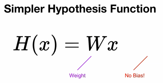
지난 번에 살펴 본 Linear Regression H(x)는 input, weight, 그리고 bias로 이루어진 식이었습니다. 이번엔, Gradient Descent에 대해 쉽게 알아보기 위해, bias가 없다고 가정한 더 간단한 Simpler Hypothesis Function을 사용하겠습니다.
Data
Cost function
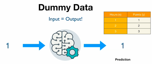
위 data에 대해서 최적의 H(X)는 w가 1일 때 즉,
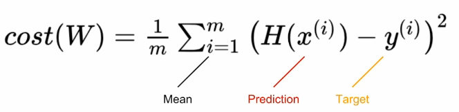
H(X) = x 일 때이다.Cost function으로는 MSE 방식을 사용할 것입니다.
Gradient Descent
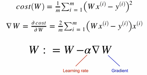
cost function을 통해 나온 cost 값을 최소화 하는 것이 우리의 목적입니다.
w가 1일 때, w와 cost의 관계를 그래프로 나타내면 아래의 그림과 같습니다.
우리는 이 함수의 그래프 상에서 cost가 가장 작아지는 지점으로 가야 하는데, 다시 말해 해당 지점에서의 기울기가 작아지는 방향으로 w를 update하는 방법이라고 할 수 있습니다.
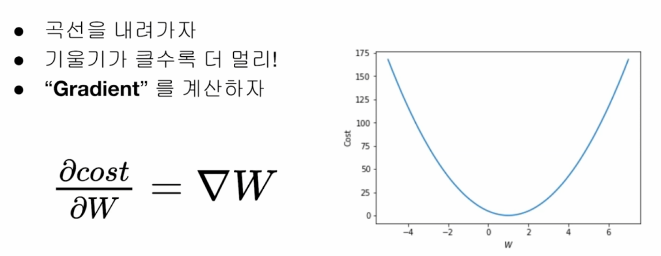
기울기를 구하기 위해선 미분을 해야 합니다. cost function의 해당 지점에서의 미분계수를 구합니다. 이 값과 얼마나 update 할 지를 결정하는 α (Learning rate)를 곱해 W에 반영합니다.
코드로 구현하면 다음과 같습니다.
gradient = 2 * torch.mean((W * x_train - y_train) * x_train)
lr = 0.1 (α)
W -= lr * gradient
정리
다음과 같이 torch 코드를 작성할 수 있습니다.
x_train = torch.FloatTensor([[1], [2], [3]])
y_train = torch.FloatTensor([[1], [2], [3]])
W = torch.zeros(1)
lr = 0.1

nb_epochs = 10
for epoch in range(nb_epochs + 1):
	hypothesis = x_train * W

    cost = torch.mean((hypothesis-y_train)**2)
    gradient = torch.sum((W * x_train - y_train) * x_train)

    print('Epoch {:4d}/{} W: {:.3f}, Cpst: {:.6f}'.format(epoch, nb_epochs, W.item(), cost.item()))

   	W -= lr * gradient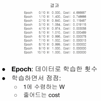
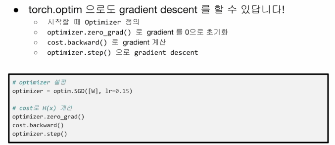
torch.optim
우리는 위에서 gradient를 직접 구현했지만, torch에는 이를 도와주는 optimizer 라이브러리가 존재한다.
x_train = torch.FloatTensor([[1], [2], [3]])
y_train = torch.FloatTensor([[1], [2], [3]])
W = torch.zeros(1)

optimizer = optim.SGD([W], lr=0.1)

nb_epochs = 10
for epoch in range(nb_epochs + 1):
	hypothesis = x_train * W

    cost = torch.mean((hypothesis-y_train)**2)

    print('Epoch {:4d}/{} W: {:.3f}, Cpst: {:.6f}'.format(epoch, nb_epochs, W.item(), cost.item()))

    optimizer.zero_grad()
    cost.backward()
    optimizer.step()

   	# W -= lr * gradient
    # 이 부분이 빠집니다. 자동으로 W update가 이뤄집니다.
What's Next?
다음부터는 여러 개의 정보에서 한 값을 예측해 볼 겁니다.