ROC

혼돈 행렬(Confusion Matrix)

• 분류 모델의 성능을 평가하는 데 사용하는 표
• 예측값과 실제값을 비교하여 모델이 얼마나 정확하게 분류했는지 확인 할 수 있음

실제 값 \ 예측 값	Positive (P)	Negative (N)	설명
Positive (P)	TP (True Positive)	FN (False Negative)	실제 Positive를 올바르게 예측
Negative (N)	FP (False Positive)	TN (True Negative)	실제 Negative를 올바르게 예측

1. 정확도(Accuracy)
   전체 데이터 중에서 올바르게 예측한 비율을 의미

   $Accuracy = \frac{TP + TN}{TP + TN + FP + FN}$

2. 정밀도(Precision)
   모델이 Positive라고 예측한 것 중에서 실제로 Positive인 비율을 의미

   $Precision = \frac{TP}{TP + FP}$

3. 재현율(Recall)
   실제 Positive 중에서 모델이 Positive라고 예측한 비율을 의미

   $Recall = \frac{TP}{TP + FN}$

4. F1-스코어(F1-Score)
   Precision과 Recall의 조화 평균으로, 두 값이 균형을 이루도록 함

   $F1\text{-}Score = \frac{2 \times Precision \times Recall}{Precision + Recall}$

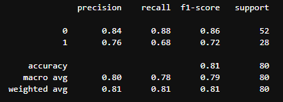
classification_report()

• Scikit-learn의 metrics 모듈에서 제공하는 분류 모델의 평가 지표를 출력해주는 함수
• classification_report()를 통해 정확도, 정밀도, 재현율, F1-스코어, Support의 값을 확인 할 수 있음

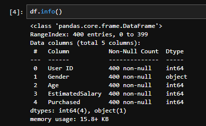
사용 cvs 정보

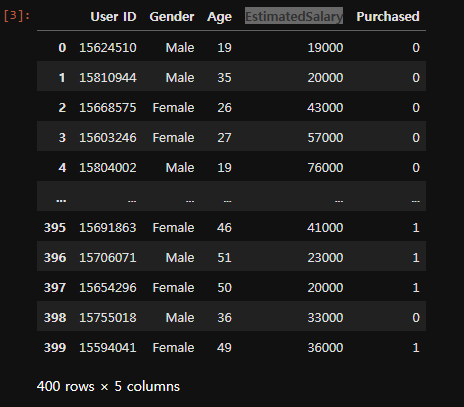
이상치 해결

• traindata에서 Age와 EstimatedSalary의 값 차이가 크기 때문에 이상치를 해결해야함

1. MinMaxScaler

minmax_scaler = MinMaxScaler()
X = minmax_scaler.fit_transform(X)
print(X)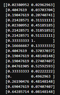

2. StandardScaler

X2 = df.loc[:, 'Age':'EstimatedSalary']

stand_scaler = StandardScaler()
X2 = stand_scaler.fit_transform(X2)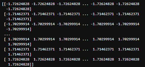

train, test 데이터 분류및 모델 학습

X = df.loc[:, 'Age':'EstimatedSalary'] # train_data
y = df['Purchased'] #target
X_train, X_test, y_train, y_test = train_test_split(X, y, test_size= 0.2)
model = LogisticRegression()
model.fit(X_train, y_train)

y_pred = model.predict(X_test)
accuracy = accuracy_score(y_test, y_pred)
print(f"Accuracy: {accuracy}")

confusion_matrix, classification_report

cm = confusion_matrix(y_test ,y_pred)
print(cm)
cr = classification_report(y_test ,y_pred)
print(cr)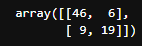

ROC Curve와 AUC

ROC Curve

• 이진 분류 모델의 성능을 평가하는 그래프

• TPR(True Positive Rate)는 Positive로 예측된 것들 중 진짜 Positive인 것의 비율을 나타냅니다.

  $TPR = \frac{TP}{TP+FN}$

• TNR(True Negative Rate)는 Negative로 예측된 것들 중 진짜 Negative인 것의 비율을 나타냅니다.

  $TNF = \frac{TN}{TN + FP}$

• ROC를 이용하여 DecisionTreeClassifier, LogisticRegression, SVC 평가

# 데이터 발생 (데이터 열기)
X, y = make_classification(n_samples = 10000, n_classes = 2, random_state = 42) #  random_state = 42로 많이 설정(약속)
tate = 42)
# 데이터 분리 
X_train, X_test, y_train, y_test = train_test_split(X, y, test_size = 0.2)

# 모델 생성 및 학습
# 데이터 생성, 데이터 훈련 테스트 분리, 모델생성/ 모델fit()/predict(x_test)
dt = DecisionTreeClassifier()
lr = LogisticRegression()
svc = SVC(probability=True)

dt.fit(X_train,y_train)
svc.fit(X_train,y_train)
lr.fit(X_train,y_train)

y_pred_dt = dt.predict_proba(X_test) # 예측보다는 성능의 비교, 입계 = 경계 threshold
y_pred_svc = svc.predict_proba(X_test)
y_pred_lr = lr.predict_proba(X_test)

fpr_dt, tpr_dt, z = roc_curve(y_test, y_pred_dt[:, 1])
fpr_svc, tpr_svc, z = roc_curve(y_test, y_pred_svc[:, 1])
fpr_lr, tpr_lr, z = roc_curve(y_test, y_pred_lr[:, 1])

plt.plot(fpr_dt, tpr_dt, color='r', label = 'DecisionTreeClassifier')
plt.plot(fpr_svc, tpr_svc, color='g', label = 'SVC')
plt.plot(fpr_lr, tpr_lr, color='b', label = 'LogisticRegression')
plt.plot([0,1], [0,1], 'k--')
plt.title('dt, svc, lr 모델 Roc커브 그래프')
plt.xlabel('False Positive Rate')
plt.ylabel('True Positive Rate')
plt.legend()
plt.show()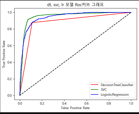

AUC

• ROC 곡선 아래 면적
• 분류 모델의 성능을 평가하는 지표
• 1에 가까울수록 모델이 좋은 성능을 보임
• 0.8이상이면 좋은 모델
  AUC 값 범위: 0 ~ 1
  AUC = 1 → 완벽한 모델 (100% 정확한 분류)
  AUC = 0.5 → 랜덤 예측과 동일한 성능 (무의미한 모델)
  AUC < 0.5 → 성능이 최악 (반대로 예측하는 경우)

# 5. AUC Area Under Curve - 
# roc_auc_score, roc_curve
auc_dt = roc_auc_score(y_test, y_pred_dt[:, 1])
auc_dt
auc_svc = roc_auc_score(y_test, y_pred_svc[:, 1])
auc_svc
auc_lr = roc_auc_score(y_test, y_pred_lr[:, 1])
auc_lr

1. auc_dt
   0.8830377893604171
2. auc_svc
   0.9526812965266749
3. auc_lr
   0.9438979803272917