이상치

Doya·2025년 3월 17일

EST_캠프_AI개발7기

ESTSOFT_AI개발7기

목록 보기

24/43

이상치(Outlier)

관측된 데이터 범위에서 많이 벗어난 아주 작은 값이나 큰값을 의미
어떤 의사결정을 하는데 필요한 데이터를 분석, 모델링 할 경우 결과 값에 큰 영향을 미칠수 있음
전처리 과정에서 이상치 처리가 필요함

이상치 판단 방법

1. IQR(Interquartile Range, 사분위수 범위)방법

데이터가 정규 분포를 따르지 않아도 적용 가능한 방법
Q1(1분위수): 데이터를 작은 값부터 정렬시 하위 25%에 해당하는 값
Q3(3분위수): 데이터를 작은 값부터 정렬시 상위 25%에 해당하는 값
IQR(사분위수 범위): Q3 - Q1
- Q1 과 Q3 사이 데이터를 집중적으로 분석할 때 사용
lower_limit = Q1 - 1.5 IQR, uppper_limit = Q1 - 1.5 IQR
- 1.5 대신 3을 곱할수도 있음. 이때는 더 극단적인 이상치만 걸러지고, 1.5보다 더 작은 값을 곱하면 더 많은 데이터를 이상치로 간주함

정규분포

대부분의 데이터가 평균 근처에 몰려있고, 평균에서 멀어질수록 데이터 개수가 점점 줄어드는 대칭적인 분포

2. Z-Score(표준 점수)방법

데이터가 정규 분포를 따를 때 효과적임
각 데이터가 평균으로부터 몇 개의 표준편차 만큼 떨어져 있는지 계산
공식 $Z = \frac{X-μ}{σ}$

X: 개별 데이터 값
μ: 평균(mean)
σ: 표준편차(std)

분산

편차의 제곱의 평균값

표준편차

데이터가 평균으로 부터 얼마나 멀리 퍼져 있는지를 측정한 값
분산의 제곱근을 의미
표준편차가 작으면 데이터는 평균 근처에 몰려있는 것이고, 크면 데이터가 평균에서 많이 벗어난 것을 의미

자전거 대여 데이터를 이용한 실습

데이터 정보

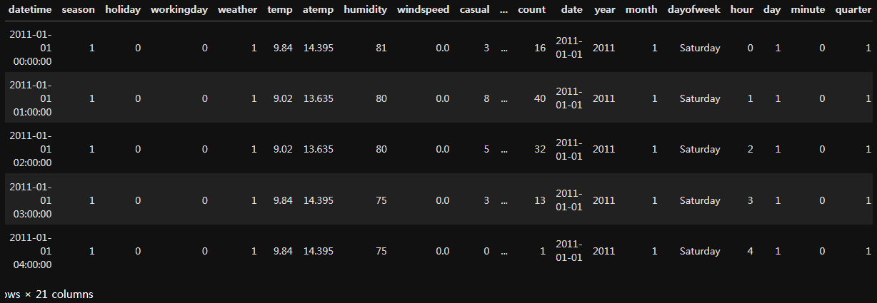
날짜 데이터 변경

# train람다식으러 변경 
train['year'] = train['datetime'].apply(lambda x : x.year)
train['month'] = train['datetime'].apply(lambda x : x.month)
train['day'] = train['datetime'].apply(lambda x : x.day)
train['date'] = train['datetime'].apply(lambda x : x.date)   
train['dayofweek'] = train['datetime'].apply(lambda x : x.day_name())
train['hour'] = train['datetime'].apply(lambda x : x.hour)
train['minute'] = train['datetime'].apply(lambda x : x.minute)
train['quarter'] = train['datetime'].apply(lambda x : x.quarter)
print( train )  

test['year'] = test['datetime'].dt.year
test['month'] = test['datetime'].dt.month
test['day'] = test['datetime'].dt.day
test['date'] = test['datetime'].dt.date
test['dayofweek'] = test['datetime'].dt.day_name()    
# test['dayofweek'] = test['datetime'].dt.day_of_week  
test['hour'] = test['datetime'].dt.hour
test['minute'] = test['datetime'].dt.minute
test['quarter'] = test['datetime'].dt.quarter
print( test )

lineplot을 이용한 시각화

train['date'] = train['datetime'].dt.date
plt.figure(figsize=(16,4))
sns.lineplot(data=train, x='date', y='count')
plt.xticks(rotation=45)
plt.title("train데이터 date lineplot test ")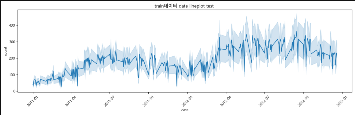

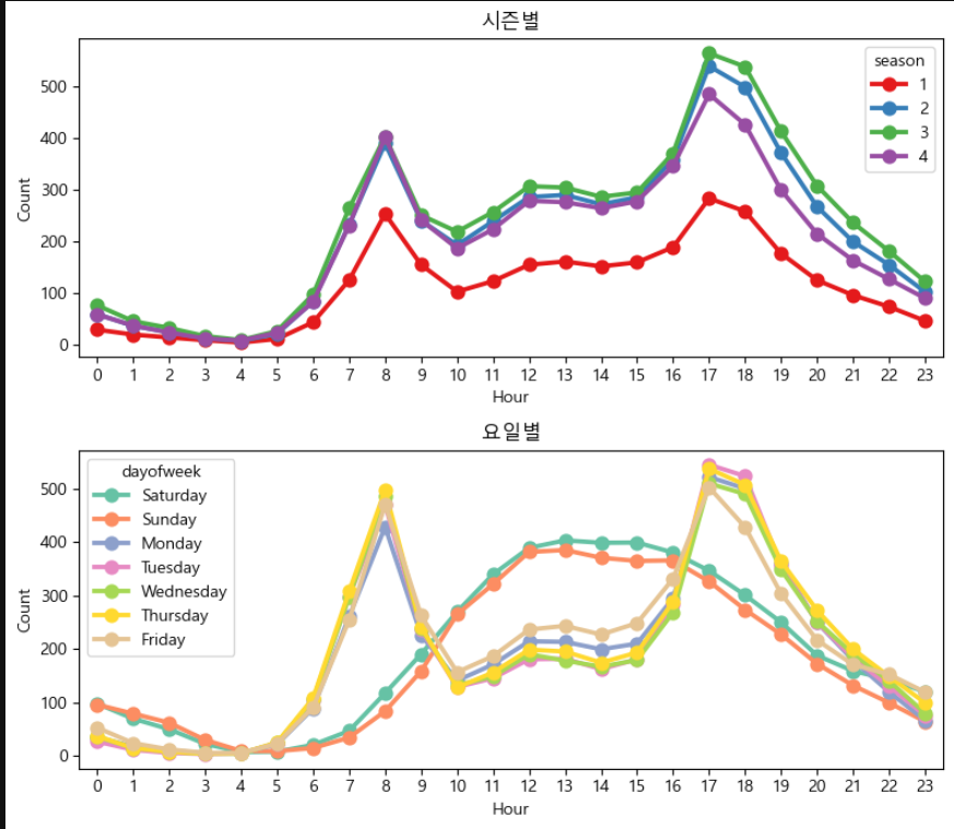
시즌별, 요일별 시각화

fig, axes = plt.subplots(2, 1, figsize=(12, 7))

sns.pointplot(data = train, x = 'hour', y = count, hue = 'season', ax = axes[0], errorbar= None, palette= 'Set1')
axes[0].set_title('시즌별')
axes[0].set_xlabel('Hour')
axes[0].set_ylabel('Count')

sns.pointplot(data = train, x = 'hour', y = count, hue = 'dayofweek', ax = axes[1], errorbar= None , palette = 'Set2')
axes[1].set_title('요일별')
axes[1].set_xlabel('Hour')
axes[1].set_ylabel('Count')

plt.tight_layout()
plt.show()

이상치 제거

Z-score

def remove_outliers_zscore(df, col, threshold=3):
    mean = df[col].mean()  # 평균
    std = df[col].std()  # 표준편차

    # Z-Score 계산
    df['z_score'] = (df[col] - mean) / std

    # 이상치 제거 (Z-Score가 절대값 threshold 이상인 경우 제거)
    filtered_df = df[np.abs(df['z_score']) < threshold].copy()
    
    # Z-Score 컬럼 삭제 (원본 데이터 유지)
    filtered_df = filtered_df.drop(columns=['z_score'])

    return filtered_df
# train 데이터 이상치 제거
train = remove_outliers(train, 'count')

from collections import Counter 
def my_dropIQR(df, n, feature):
    outer = []
    for col  in feature:
        Q1 = np.percentile(df[col], 25)
        Q3 = np.percentile(df[col], 75)
        IQR = Q3 - Q1 
        step = 1.5 * IQR
        outer_col = df[ (df[col] < Q1 - step) | (df[col] > Q3 + step) ].index
        outer.extend(outer_col)
    outer = Counter(outer)
    ret = list( k for k,v in outer.items() if v < n) 
    return ret
    
outdrop = my_dropIQR(train, 2, ['count', 'registered'])
train = train.drop(outdrop, axis = 0).reset_index(drop = True)

[10886 rows x 20 columns] => [10669 rows x 21 columns] 이상치 제거

데이터 학습

X_train = train[categorical_feature_names]
X_test = test[categorical_feature_names]
label_name = 'count'
y_train = train[label_name]

model = RandomForestRegressor(n_estimators = 100, random_state = 42)
print(model)

model.fit(X_train, y_train)
y_pred = model.predict(X_test)
print(f'예측값  {y_pred[ : 10]}')