✅ Multi-Layer Perceptron (NN)

• 은닉층이 두개 이상인 신경망 구조
• XOR 문제를 해결 할 수 있다.
  (앞선 퍼셉트론 하나로는 해결할 수 없었잖아:))

데이터 입출력 정의

import torch

torch.manual_seed(777)

X = torch.FloatTensor([[0,0], [0,1], [1,0],[1,1]])
Y = torch.FloatTensor([[0],[1],[1],[0]])

앞선 실습과 동일한 data야!

NN 모델 정의

• Perceptron과 차이는 모델 설계 부분

## 모델 설계
layer1 = torch.nn.Linear(2,2,bias=True)
layer2 = torch.nn.Linear(2,1,bias=True)
sigmoid = torch.nn.Sigmoid()

아까는 layer가 1개밖에 없었다구! 근데 이번에는 layer이 2개야

model = torch.nn.Sequential(layer1,sigmoid,layer2,sigmoid)
model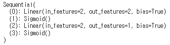

모델 학습

loss = torch.nn.BCELoss()
optimizer = torch.optim.SGD(model.parameters(), lr=1)

이진분류문제이기 때문에 여전히 BCELoss

for stop in range(10000):
    
    # 그래디언트 초기화
    optimizer.zero_grad()
    # Forward 계산
    hypothesis = model(X)
    # Error 계산
    cost = loss(hypothesis, Y)
    # Backward 계산 
    cost.backward()
    # 가중치 갱신
    optimizer.step()

    if stop % 100 == 0:
        print(stop, cost.item())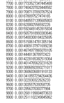

모델 평가

## w,b 평가

with torch.no_grad(): # 임시로 required_grad = false로 설정하는 것과 같다.

    hypothesis = model(X)
    predicted = (hypothesis > 0.5).float() # logistic regression => binary classification
    accuracy = (predicted == Y).float().mean()
    print('\n Hypothesis: ', hypothesis.numpy(), '\n Correct: ', predicted.numpy(), '\n Accuracy: ', accuracy.item())

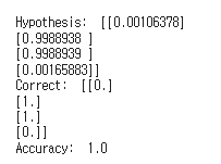앞선 퍼셉트론 1개였을 때는 accuarcy가 0.5였는데 2개를 쌓으니 1로 완벽하게 XOR문제를 해결하는 것을 볼 수 있었지.

🟢 모델을 더 깊게 쌓은 실험

다른건 다 동일하고 이 부분만 바꾼 것!

NN 모델 정의

• 더 넓고, 깊게 만들기
  - 깊게: 은닉층 늘리기
  • 넓게: features 수 늘리기

## 모델 설계
linear1 = torch.nn.Linear(2, 10, bias=True)
linear2 = torch.nn.Linear(10, 10, bias=True)
linear3 = torch.nn.Linear(10, 10, bias=True)
linear4 = torch.nn.Linear(10, 1, bias=True)
sigmoid = torch.nn.Sigmoid()

model = torch.nn.Sequential(linear1, sigmoid, linear2, sigmoid, linear3, sigmoid, linear4, sigmoid)

여기서는 그렇게 적용하지 않았는데 (이후의 강의에서는) 마지막 layer에서는 활성화함수를 빼는게 좋다고 하시기는 하셨거든..? 이후에 더 한번 봐야할 것 같다

• 추가로 bias=True가 default값이기 때문에 굳이 할 필요 없기는 했어

모델 학습

for stop in range(10000):
    
    # 그래디언트 초기화
    optimizer.zero_grad()
    # Forward 계산
    hypothesis = model(X)
    # Error 계산
    cost = loss(hypothesis, Y)
    # Backward 계산 
    cost.backward()
    # 가중치 갱신
    optimizer.step()

    if stop % 100 == 0:
        print(stop, cost.item())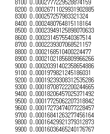

아까보다 loss값이 확연히 줄어든 것을 볼 수 있었어

모델 평가

## w,b 평가

with torch.no_grad(): # 임시로 required_grad = false로 설정하는 것과 같다.

    hypothesis = model(X)
    predicted = (hypothesis > 0.5).float()
    accuracy = (predicted == Y).float().mean()
    print('\n Hypothesis: ', hypothesis.numpy(), '\n Correct: ', predicted.numpy(), '\n Accuracy: ', accuracy.item())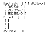

이미 아까 accuarcy로 1이었기 때문에 정말 성능이 향상되었나 싶을 수도 있지만 loss값이 줄어들었잖아 충분히 성능 향상이지 :)