24.02.05 TIL

오늘은 그래도 과제 해설이 유익했다.
아예 모르는 건 알려줘도 못 먹어서 아쉽지만,,
더 공부해야지 모

---

<데이터 전처리 - 이상치 >

1. Extreme Studentized Deviation(ESD) 이용한 이상치 발견

• 데이터가 정규분포를 따른다고 가정할 때, 평균에서 표준편차의 3배 이상 떨어진 값
• 모든 데이터가 정규 분포를 따르지 않을 수 있기 때문에 데이터가 크게 비대칭일 때( → Log변환), 샘플 크기가 작을 경우에는제한됨

1. IQR(Inter Quantile Range)를 이용한 이상치 발견

• Box plot: 데이터의 사분위 수를 포함하여 분포를 보여주는 시각화 그래프, 상자-수염 그림이라고도 함
  • 사분위 수: 데이터를 순서에 따라 4등분 한 것
  • $Q1(25\%), Q2(50\%,중위수), Q3(75\%)$
  • $IQR(Inter \ quantile \ range) = Q3 - Q1$
  • $상한 \ 이상치 = Q3 + 1.5*IQR \\ 하한 \ 이상치 = Q1 - 1.5*IQR$
• ESD를 이용한 처리

import numpy as np
mean = np.mean(data)
std = np.std(data)
upper_limit = mean + 3*std
lower_limit = mean - 3*std

• IQR을 이용한 처리(box plot)

Q1 = df['column'].quantile(0.25)
Q3 = df['column'].qunatile(0.75)
IQR = Q3 - Q1
uppper_limit = Q3 + 1.5*IQR
lower_limit = Q1 - 1.5*IQR

• 조건필터링을 통한 삭제(a.k.a. boolean Indexing): df[ df['column'] > limit_value]

  - 데이터를 True/False로 나눠 보고싶은 값만 보게 하는 방법

** 이상치는 비즈니스 맥락에 따라 기준이 달라지며 정보 손실을 동반하므로 주의 필요

** 이상 탐지(Anomaly Detection) 등의 패턴을 다르게 보이는 개체 또는 자료를 찾는 방법으로도 발전 가능

<데이터 전처리 - 결측치 >

결측치(Missing Value) : 존재하지 않는 데이터

• 결측치 처리 방법

  • 수치형 데이터(기술통계)

    • 평균값 대치: 대표적인 대치 방법
    • 중앙값 대치: 데이터에 이상치가 많아 평균 값이 대표성이 없다면 중앙 값을 이용 Ex) 이상치는 평균 값을 흔들리게 함

  • 범주형 데이터
    - 최빈값 대치

    ** 다변량 대치 : 결측이 된 값을 Y값이라고 생각, 결측 외에 나머지 값을 통해 Y에 들어갈 값을 예측하고, 전체의 값을 X로 생각하고 또 Y를 예측하는 (예측의 예측) 방법

    ** 알고리즘 익혀두면 수치형 데이터 스케일링 할 때 계속 쓰임

• EDA

import seaborn as sns
import matplotlib.pyplot as plt 
import pandas as pd

tips_df = sns.load_dataset('tips')
tips_df.head()

tips_df.describe(include = 'all')

#countplot: x축 범주형, y축 관측치
sns.countplot(data = tips_df, x = 'day')

#barplot : x축 범주형, y축 연속형 값
sns.barplot(data = tips_df, x = 'sex', y = 'tip', estimator = 'mean')

#Boxplot : 이상치 확인 가능
sns.boxplot(data = tips_df, x = 'time', y = 'total_bill')

#histplot: 히스토그램 / bins = 그래프 개수
sns.histplot(data = tips_df, x = 'total_bill', bins = 20)

tips_df['total_bill'].hist()
tips_df['total_bill'].plot.hist()

#x축 : 수치형변수 / y축 : 수치형변수
sns.scatterplot(data = tips_df, x = 'total_bill', y = 'tip')

sns.pairplot(data = tips_df)

• 이상치

#ESD를 이용한 이상치 확인
import numpy as np 
mean = np.mean(tips_df['total_bill'])
std = np.std(tips_df['total_bill'])
upper_limit = mean + 3*std
lower_limit = mean - 3*std
print(upper_limit, lower_limit)

tips_df[['total_bill']].head(3)

cond = (tips_df['total_bill'] > 46.4)
cond

tips_df[cond]

#IQR을 이용한 이상치 확인
sns.boxplot(tips_df['total_bill'])

q1 = tips_df['total_bill'].quantile(0.25)
q3 = tips_df['total_bill'].quantile(0.75)
iqr = q3 - q1
upper_limit2 = q3 + 1.5*iqr
lower_limit2 = q1 - 1.5*iqr
print(q1, q3, iqr, upper_limit2, lower_limit2)

cond2 = (tips_df['total_bill'] > upper_limit2)
tips_df[cond2]

• 결측치

import pandas as pd

titanic_df = pd.read_csv('/Users/yejin/Documents/ML 실습/train-2.csv')

titanic_df.head(3)

titanic_df.info()

titanic_df.dropna(axis = 0).info()

cond3 = (titanic_df['Age'].notna())
titanic_df[cond3].info()

#fillna를 이용한 대치
age_mean = titanic_df[['Age']].mean().round(2)
titanic_df['Age_mean'] = titanic_df['Age'].fillna(age_mean)

titanic_df.info()

- SimpleImputer를 이용한 대치 (평균대치)
from sklearn.impute import SimpleImputer
si = SimpleImputer()
si.fit(titanic_df[['Age']])

si.statistics_

titanic_df['Age_si_mean'] = si.transform(titanic_df[['Age']])

titanic_df.info()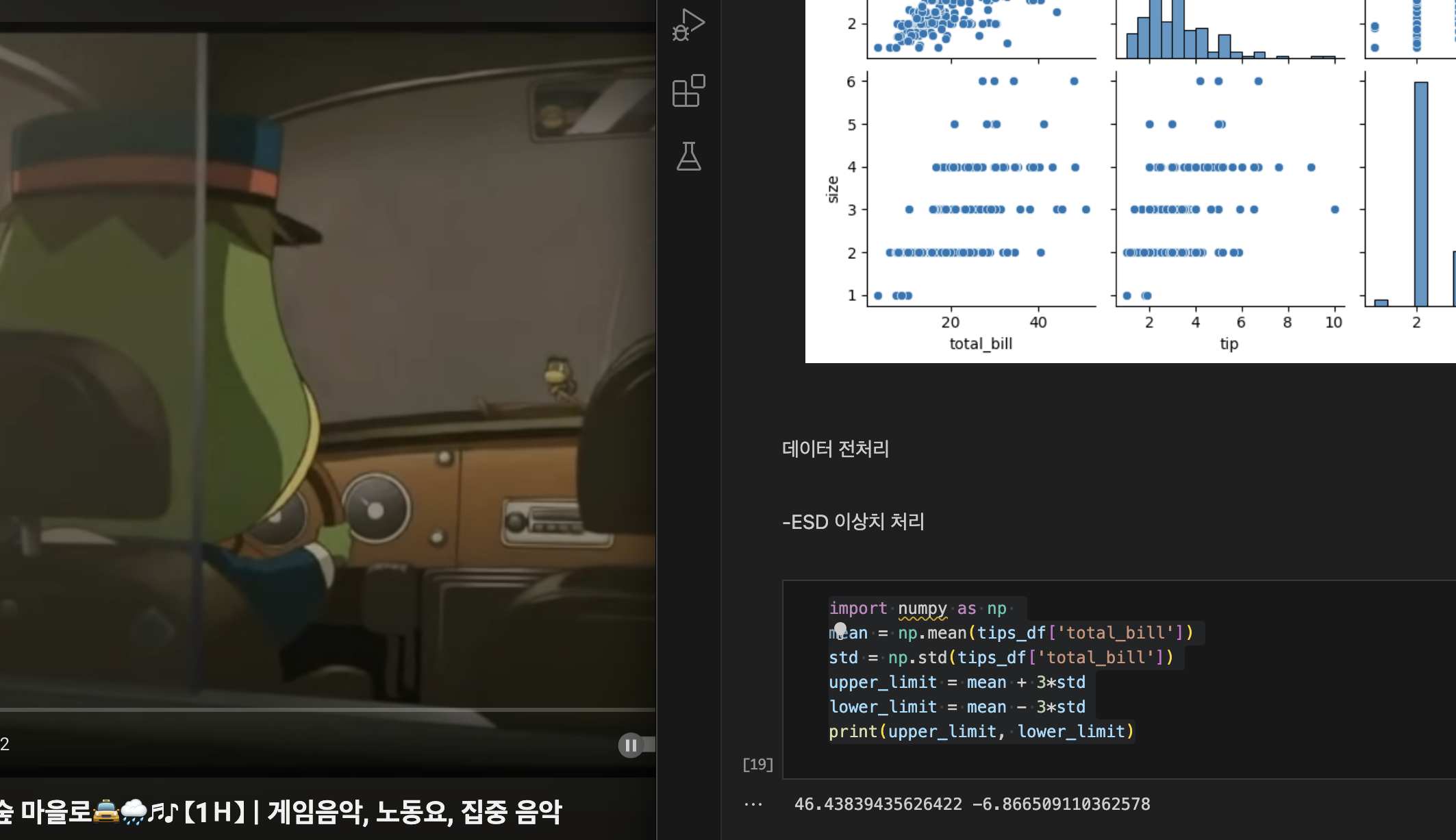

---

오늘은 할말 없.
내일부터 심화프로젝트 시작
할 수 있는 일을 하자 🫥